Updated August 11, 2023
Excel Accounting Number Format (Table of Contents)
- Accounting Number Format in Excel
- Difference between Currency and Accounting Number Format in Excel
- How to use Accounting Number Format in Excel?
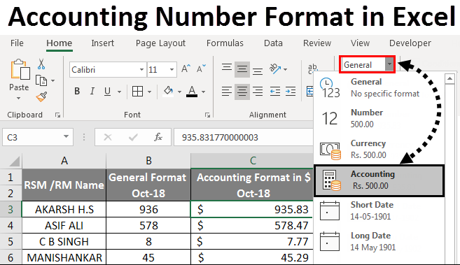
Accounting Number Format in Excel
The accounting number format in Excel consists of numbers with the involvement of currency. For example, if you enter the currency name manually with any number manually, the cell value becomes General or Text. And the number of currency cannot be used anywhere. To make that number accountable, click right and select Format Cells and the Accounting section and select the needed currency. We will see, the number will have a currency symbol, and that cell value is still countable in all the financial work.
Difference Between Currency and Accounting Number Format in Excel
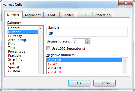
Currency Format
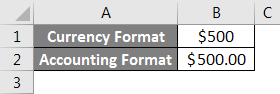
The currency format is one of the number formattings in excel, which places the dollar $ sign on the right side to the number. For example, if we format the number 500 to currency format, Excel will display the output as $500. We can convert the number to currency format by simply clicking the currency number format in the number group, or we can use the shortcut key as CTRL+SHIFT+$
Accounting Format
The Accounting format is also one of the number formattings in excel, which aligns the dollar sign at the left edge of the cell and displays it with two decimal points. For example, if we format the number to Accounting format, Excel will display the output as $500.00. We can convert the number to accounting format by simply clicking the accounting number format in the number group, and if there are any negative numbers accounting format will display the out in parenthesis $ (500.00)
The difference between Currency and Accounting format is shown in the below screenshot.
How to Use Accounting Number Format in Excel?
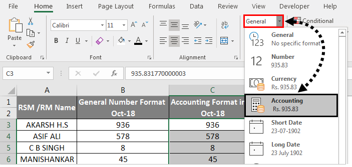
In Microsoft Excel, we can find the accounting format under the number formatting group shown in the below screenshot.
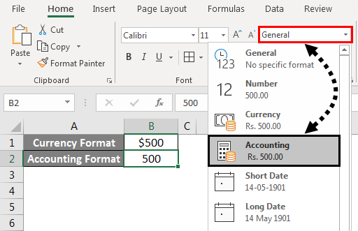
We can format the number to accounting format either by choosing the accounting option in the Number group or by right-clicking on the menu. We will see both the option in the below example.
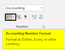
Also, we can format the number in accounting format by choosing the dollar sign $ in the number group, which is also one of the shortcuts for the accounting number format shown in the below screenshot.
Example #1
Converting Number to Excel Accounting Format
In this example, we will learn how to convert the normal number to accounting format. Consider the below example, which shows MRP, Selling Price of the individual product with local, national and zonal prices.
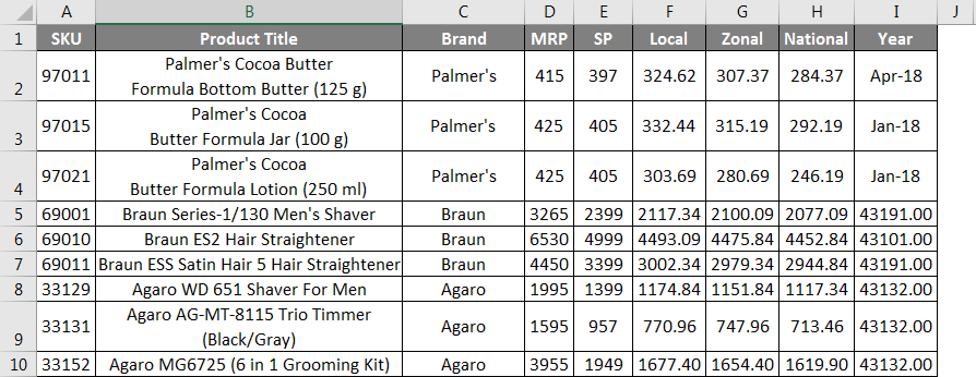
As we can notice that all the numbers are in general format by default, Assume that we need to convert the “Selling Price” to Accounting Number format along with Local, Zonal, and National selling prices.
In order to convert the number to Accounting format, follow the below procedure step by step.
- First, select the column from E to H, where it contains the product’s selling price, which is shown in the below screenshot.

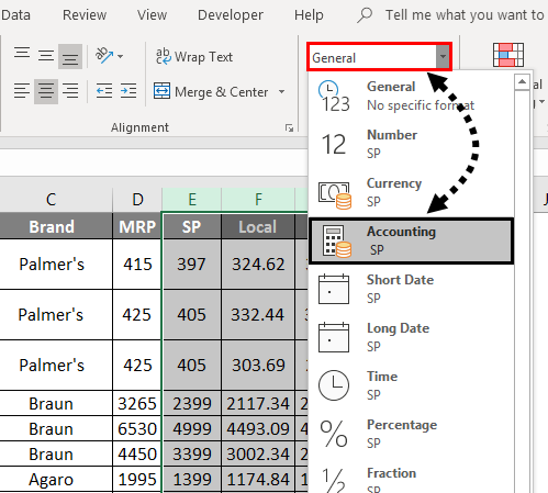
- Now go to the Number group option and click on the drop-down box. In the drop-down list, we can see the Accounting format option.
- Click on the Accounting number format.
- Once we choose the Accounting number format, we will get the output as ###, which is shown below.
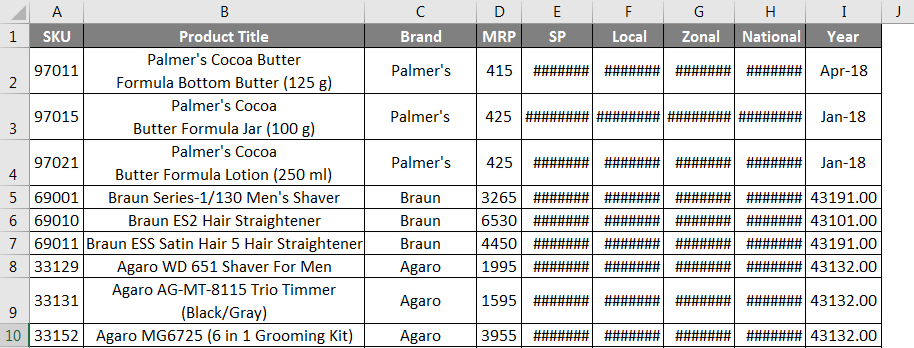
- We can notice that once we convert the number to accounting number format, excel will align the dollar sign at the left edge of the cell and display with two decimal points that we are getting the ### hash symbols.
- Enlarge all the columns so that we can see the exact accounting format output, which is shown below.
In the below result, we can see that all the numbers are converted where we can see the Dollar sign$ in each left edge of the cell separated by commas and with two decimal numbers.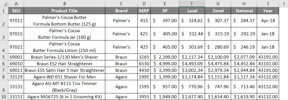
Example #2
Converting Number to Accounting format using Right-Click Menu
In this example, we are going to see how to convert a number using the right-click menu. Consider the same above example, which shows MRP, selling the product with local, national, and zonal prices. We can increase or decrease the decimal places by clicking the “Increase Decimal” and “Decrease Decimal“ icons at the number group.
To apply accounting number formatting, follow the below step by step procedure as follows.
- First, select the column from E to H, where it contains the product’s selling price, which is shown in the below screenshot.

- Now Right-click on the cell so that we will get the below screenshot which is shown below.

- Click on the Format Cells so that we will get the number formatting dialog box which is shown below.
- In the above screenshot, we can see the list of number formatting options.
- Select the Accounting option so that it will display the accounting format, which is shown below.
- As we can see, on the right-hand side, we can see decimal places where we can increase and decrease the decimal points, and next to that, we can see the symbol drop-down box, which allows us to select which symbol needs to be displayed. (By default, accounting format will select the Dollar Sign $)
- Once we increase the decimal places, the sample column will display the number with selected decimal numbers which are shown below.
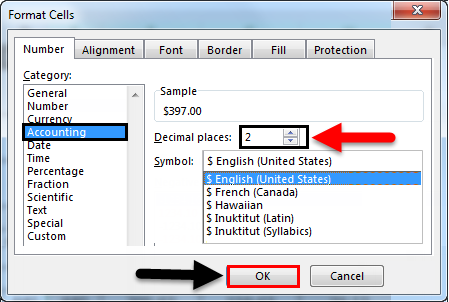
- Click the OK button so that the selected selling price column will get converted to Accounting number format, which is shown as a result in the below screenshot.
Example #3
This example shows how to sum the accounting number format by following the below steps.
Consider the example which shows sales data for the month of OCT-18.

As we can see that there are normal sales figures in the General number format. Now we will convert the above sales figure to accounting format for accounting purposes.
- First, copy the same B column sales figure next to the C column, which is shown below.
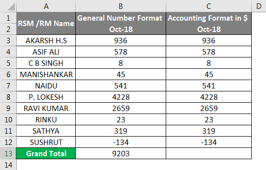
- Now select the C column and go to the number formatting group and choose Accounting, shown below.
- Once we click on the accounting format, the selected numbers will be converted to Accounting format, shown below.
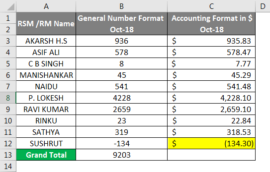
- As we can see, the difference that C column has been converted to accounting format with a Dollar sign with two decimal places and at the last column for negative numbers accounting format has shown the number inside the parenthesis.
- Put the SUM formula in the C13 column, which will show the SUM in accounting format.
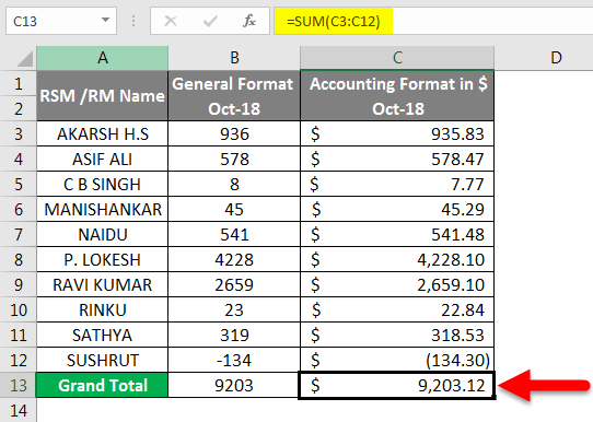
In the below result, we can see that the accounting format which automatically uses the dollar sign, decimal places, and comma to separate a thousand figures where we cannot see those in General number format.
Things to Remember
- The accounting number format is normally used for financial and accounting purposes.
- The accounting number format is the best way to configure the values.
- For negative values accounting format will automatically insert the parenthesis.
Recommended Articles
This has been a guide to Accounting Number Format in Excel. Here we discussed how to use Accounting Number Format along with practical examples and a downloadable excel template. You can also go through our other suggested articles –