Updated June 9, 2023
Introduction to EOMONTH Formula
To understand the EOMONTH Formula in Excel, we first need to know what it means in simple language and why we need this function. Here the term “EO” means “End Of,” and EOMONTH means “End Of Month”. To determine the end of the respective month of a given date in Excel, we use the EOMONTH function.EOMONTH Function in Excel comes under the date and time function in MS Excel.
It helps to search the last day of the month for the current month, past months, and future months from a particular date. It helps compute maturity dates for Creditors or Bills Payable and Creditors or Bills Payable that are effective on the last day of the month or at the end of the month.
Syntax
Arguments of EOMONTH formula:
- Start _date – It is the given date. The specific format should follow while entering the initial date, such as “mm/dd/yyyy”, the default format. Otherwise, we can use a customized format. Or we can also use the DATE Function, which also comes under the DATE AND TIME Function, to avoid getting an ERROR such as #NUM! OR #VALUE!
- months – It is always a numerical value to specify how many months before or after the specifieMonths n “Start _ Date”. It can be 0, any positive whole number, or any negative whole number.
How to Use the EOMONTH Formula?
EOMONTH Formula in Excel is very simple and easy. Let’s understand how to use the EOMONTH Formula in Excel with some examples. We will discuss 2 examples of the EOMONTH Function. 1st one is for the data in a Vertical Array, and the later one is for the data in a Horizontal Array.
Example #1
To understand the EOMONTH Function, let us take one example.
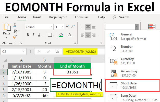
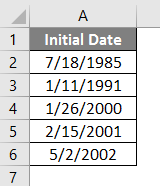
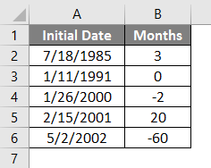
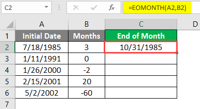
Bruce Banner wants to find the last day of the month for the given dates after considering the no. of the month in the current, past, or future. So, Bruce writes done the dates.
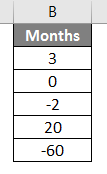
Then he writes down the no. of the month required with 0, positive or negative whole numbers.
Now he has a list of Dates with their respective no. of months to use.
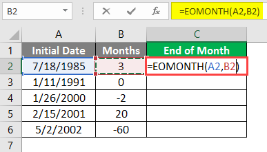
If Bruce Banner wants to find the last day of the month, he can use the EOMONTH Function. In the C3 cell, he adds EOMONTH Function, =EOMONTH(A2, B2). Where A2 is the start date. B2 is the no. of months required with 0, positive or negative whole numbers.
Therefore the result is displayed in numerical values.
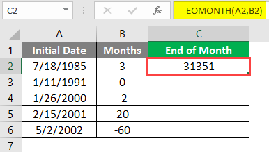
To convert it in date format, we need to follow the following steps,
Select cell C2 – go to the Home tab under the Numbers group -click on the dropdown menu to select Short date.
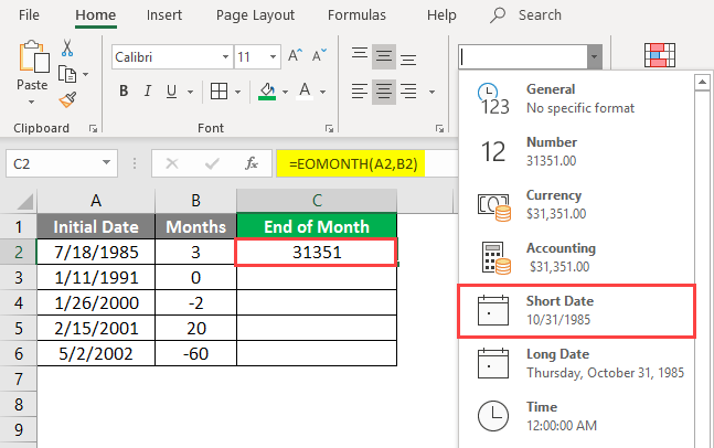
Therefore the result in date format is displayed.
Now Bruce drags down or copies the formula in other cells.
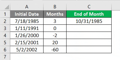
Bruce gets all the required end of month dates.
Example #2
Let us take another example of EOMONTH while calculating the Credit Period of the creditors by considering the last day of the month from the date given to the bill date of the transaction.
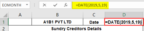
Let us consider a company named A1B1 Pvt Ltd. Scarlett Johansson, a Financial Analyst, wants to find out the creditor aging analysis. She needs to know it based on the month’s last date.
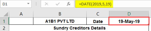
So, to achieve that, she needs to record the creditor’s details in MS Excel. She enters the details of the bill date, the Creditors Name, bill number, and the bill amount. Now in cell D1, She enters a date, for example, 19th May 2019. She uses the DATE function so that there will be no #VALUE! Error for an unidentified date value. She enters = DATE (2019, 05, 19).
Therefore date 19th May 2019 is displayed in cell D1.
She needs to check the difference in date between the bill date and the last day of the given date.
She wants to find in 3 categories less than 30 days, 31-60 days, and more than 61 days.
![]()
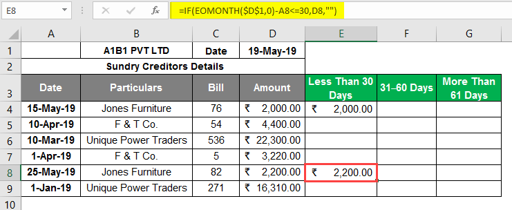
1. To find the data of “less than 30 days” in cell E4, she enters a value of the IF function,
=IF(EOMONTH($D$1,0)-A4<=30,D4,””)
Where,
D1 is the date given.
A4 is the Bill Date.
D4 is the bill value.
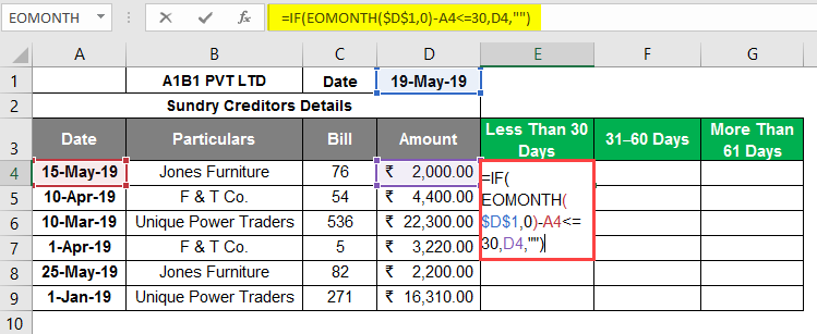
Therefore, the bill value will get displayed if the condition satisfies. Then, she must drag down the formula in case of other creditors.
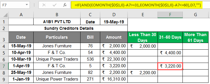
2. To find the data of “31 – 60 days” in cell F4, she enters a value of IF as well as AND functions,
=IF(AND(EOMONTH($D$1,0)-A5>=31,EOMONTH($D$1,0)-A5<=60),D5,””)
Where,
D1 is the date given.
A4 is the Bill Date.
D4 is the bill value.
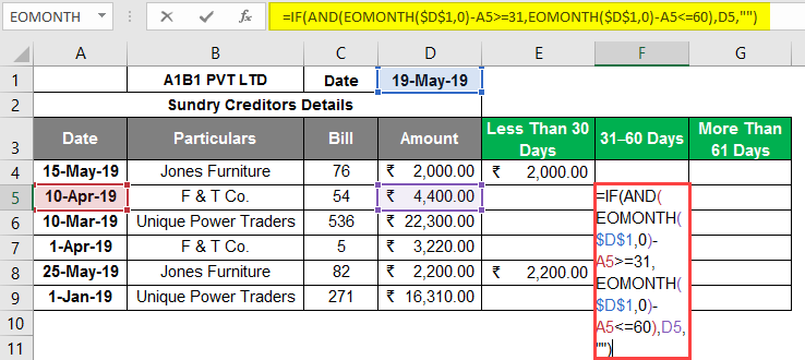
Therefore, the bill value will get displayed if the condition satisfies. Then, she must drag down the formula in case of other creditors.
3. Lastly, to find the data of “more than 61 days” in cell G4, she enters a value of the IF function,
=IF(EOMONTH($D$1,0)-A6>=61,D6,””)
Where,
D1 is the date given.
A4 is the Bill Date.
D4 is the bill value.
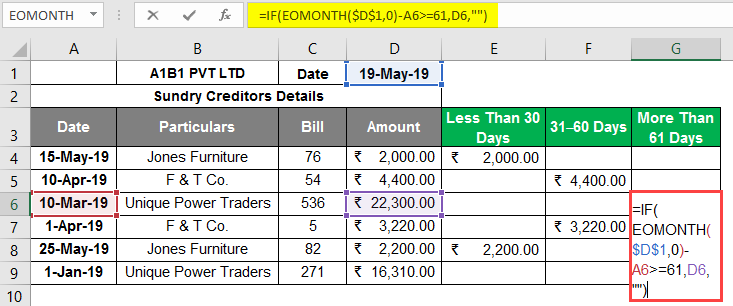
Therefore, the bill value will get displayed if the condition satisfies. Then, she must drag down the formula in case of other creditors.
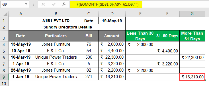
This helps Scarlett to get a clear picture of where the creditors of A1B1 Pvt Ltd stand and make creditor’s range of payment.
In this case, Unique Power Traders, both bill payments should be cleared immediately.
Things to Remember About EOMONTH Formula in Excel
- Proper dates to be given to avoid # value! Error.
- The date function can use, so there may be no invalid dates due to format.
- If the value is in decimal in the month’s argument, it will take only the positive or negative integer, not the decimal digits.
Recommended Articles
This is a guide to EOMONTH Formula in Excel. Here we discuss How to use EOMONTH Formula in Excel, practical examples, and a downloadable Excel template. You can also go through our other suggested articles –