Updated March 27, 2023
Introduction to Deep Learning Model
Deep learning models usually consume a lot of data, the model is always complex to train with CPU, GPU processing units are needed to perform training. So when GPU resource is not allocated, then you use some machine learning algorithm to solve the problem. Deep learning models would improve well when more data is added to the architecture. Deep Learning models can be trained from scratch or pre-trained models can be used. Sometimes Feature extraction can also be used to extract certain features from deep learning model layers and then fed to the machine learning model.
How to Create Deep Learning Model?
Deep Learning Model is created using neural networks. It has an Input layer, Hidden layer, and output layer. The input layer takes the input, the hidden layer process these inputs using weights that can be fine-tuned during training, and then the model would give out the prediction that can be adjusted for every iteration to minimize the error. For example, you can create a sequential model using Keras whereas you can specify the number of nodes in each layer.
Example:
from keras.models import Sequential

from keras.layers import Dense

model = Sequential()

model.add(dense(10,activation='relu',input_shape=(2,)))

model.add(dense(5,activation='relu'))

model.add(dense(1,activation='relu'))
The activation function allows you to introduce non-linearity relationships. You can specify the input layer shape in the first step wherein 2 represents no of columns in the input, also you can specify no of rows needed after a comma. The output layer has only one node for prediction. The purpose of introducing an activation function is to learn something complex from the data provided to them. This function should be differentiable, so when back-propagation happens, the network will able to optimize the error function to reduce the loss for every iteration. Weights are multiplied to input and bias is added.
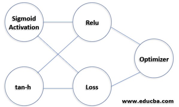
Functions of Deep Learning
Here are the functions which we are using in deep learning:
1. Sigmoid Activation Function
The function is of the form f(x) = 1/1+exp(-x). The output lies between 0 and 1. It’s not zero centered. The function suffers from vanishing gradient problem. When back-propagation happens, small derivatives are multiplied together, as we propagate to the initial layers, the gradient decreases exponentially.
2. Hyperbolic Tangent Function(tan-h)
The function is of the form f(x) = 1-exp(-2x)/1+exp(2x) . The output lies between -1 and +1. Its zero centered. Optimization convergence is easy when compared to Sigmoid function, but the tan-h function still suffers from vanishing gradient problem.
3. Relu(Rectified Linear Units)
The function is if form f(x) = max(0,x) 0 when x<0, x when x>0. Relu convergence is more when compared to tan-h function. The function does not suffer from vanishing gradient problem. It can be used only within hidden layers of the network. Sometimes the model suffers from dead neuron problem which means a weight update can never be activated on some data points. In that leaky Relu function can be used to solve the problems of dying neurons. So it’s better to use Relu function when compared to Sigmoid and tan-h interns of accuracy and performance.
Next model is complied using model.compile(). It has parameters like loss and optimizer. Loss functions like mean absolute error, mean squared error, hinge loss, categorical cross-entropy, binary cross-entropy can be used depending upon the objective function. Optimizer functions like Adadelta, SGD, Adagrad, Adam can also be used.
4. Loss Functions
Here are the types of loss functions explained below:
- MAE(Mean Absolute Error): It is one of evaluation metric which calculates the absolute difference between predicted and actual values. Take the sum of all absolute differences and divide it by the number of observations. It does not penalize large values so high as compared to MSE, which means that they are sensitive to outliers.
- MSE(Mean Squared Error): MSE is calculated by the sum of squares of the difference between predicted and actual values and dividing it by the number of observations. It needs attention when the metric value is higher or lower. Useful only when we unexpected values for predictions. We cannot rely on MSE because sometimes when the model is performing well, it may have a high MSE.
- Hinge Loss: This function is mostly used in support vector machines. The function is of form =[0,1-yf(x)]. when yf(x)>=0 the loss function is 0, but when yf(x) < 0 the error increases exponentially penalizing more to the mis-classified points that are distant from the margin. So the error would increase exponentially to those points.
- Cross-Entropy: Its a log function that predicts value lies between 0 and 1. It measures the performance of a classification model. thus when the value is 0.010 the cross-entropy loss is more and the model is bad in terms of prediction. For binary classification, cross-entropy loss is defined by -(ylog(p)+(1-y)log(1-p)). For Multi Classification, the cross-entropy loss is defined by summations of -ylog(p).
5. Optimizer Functions
Here are the types of optimizer functions explained below:
- SGD: Stochastic Gradient Descent has a problem with convergence stability. Local Minimum problem arises here. There is more fluctuation in loss functions therefore calculating the global minimum is a tedious task.
- Adagrad: Here in this Adagrad function, there is no need to manually tune the learning rate. But the main disadvantage is that the learning rate keeps on decreasing. So when the learning rate is shrinking too much for every iteration the model does not acquire additional knowledge after that. This decreasing learning rate is solved in Adadelta.
- Adadelta: Here decreasing learning rate is being solved, different learning rates are calculated for every parameter and momentum is being calculated. But the main thing is that this will not store individual momentum levels for each parameter. This problem is rectified in Adam’s optimizer function.
- Adam(Adaptive Moment Estimation): Convergence rates are high when compared to other adaptive models. Takes care of adaptive learning rates for every parameter. Mostly used in all deep learning models as momentum is also considered for each parameter. Adam’s model is very efficient and high speed. So the model can be trained with the model.fit() function where you can specify the training x parameters and y parameter, no of epochs to run, training, and testing data split. Finally, the model.predict() function would predict the outcome when sample input is passed into this function.
Conclusion
So finally the deep learning model helps to solve complex problems whether the data is linear or nonlinear. The model keeps acquiring knowledge for every data that has been fed to it.
Recommended Articles
This is a guide to Deep Learning Model. Here we discuss how to create a Deep Learning Model along with a sequential model and various functions. You can also go through our suggested articles to learn more –
