A* (star) Search Algorithm

Introduction to A star algorithm

The A* algorithm, extensively utilized in computer science, especially in artificial intelligence and game development, adeptly discovers the shortest path between two points. It achieves this by factoring in the distance from the starting point and the anticipated distance to the goal. The algorithm manages a priority queue of nodes to explore, arranged by the sum of the actual cost from the start to the current node and the anticipated cost from the current node to the goal. At each iteration, the algorithm chooses the node with the lowest total cost, expands it, and includes its neighbors in the queue.

The key to the A* algorithm’s efficiency is the heuristic function used to estimate the cost of the goal. An excellent heuristic function should be admissible, which never overestimates the actual cost. It is consistent, meaning that the estimated cost between any two nodes is equivalent to or less than the sum of the expected cost from the second node to the goal. The A* algorithm has many applications, from video game pathfinding to transportation system route planning. Its ability to find the optimal path while considering the trade-off between distance and estimated cost makes it valuable in many problem-solving scenarios.

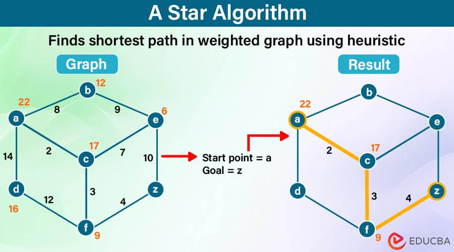
Table of Contents

• Introduction to A star algorithm
  • Understanding the A star Algorithm
  • Implementing the A star Algorithm
  • Advantages of A star Algorithm
  • Limitations of A star Algorithm
  • Real-World Applications

Understanding the A-star Algorithm

The A* (pronounced “A-star”) algorithm is a popular and widely used pathfinding algorithm in computer science and artificial intelligence. It’s especially renowned for its efficiency and effectiveness in identifying the shortest path between two points on a graph or grid while considering both the cost of reaching a particular node and estimating the remaining cost to achieve the goal.

Key Components of the A-star Algorithm

• Goal-Directed Search: A* is an informed or heuristic search algorithm. Unlike uninformed search algorithms like breadth-first search or depth-first search, A* leverages information about the goal to guide its search process more efficiently.
• Heuristic Function (h): A* utilizes a heuristic function to approximate the cost from the current node to the goal node. This heuristic function provides an optimistic estimate of the remaining cost, often denoted as h(n). A* must have an admissible heuristic, meaning it never overestimates the price to reach the goal. Common heuristics include Manhattan distance, Euclidean distance, and Chebyshev distance in grid-based environments.
• Cost Function (g): Besides the heuristic function, A* considers the cost incurred from the start node to the current node. This actual cost, denoted as g(n), is cumulatively updated as the algorithm progresses through the graph.
• F Score (f): A* combines the cost function (g) and the heuristic function (h) to evaluate the potential of each node. We calculate the f-score of a node as f(n) = g(n) + h(n). Nodes with lower f-scores are prioritized for exploration since they should lead to the shortest path.
• Open and Closed Lists: A* maintains two lists of nodes during its execution. The open list comprises nodes we have yet to explore, while the closed list contains nodes already evaluated. The algorithm repeatedly selects the node with the lowest f-score from the open list, expands it by considering its neighbors, and updates the cost and heuristic values accordingly.
• Optimality and Completeness: A* guarantees optimality (finding the shortest path) under certain conditions, such as having an admissible heuristic and non-negative edge costs. Additionally, A* is complete, meaning it will always find a solution if one exists.

Implementing the A-star Algorithm

Pseudocode

function AStar(startNode, goalNode)
    openSet := {startNode}     // Initialize the open set with the start node
    closedSet := {}            // Initialize the closed set as empty
    gScore[startNode] := 0    // Cost from start along the best known path
    fScore[startNode] := gScore[startNode] + heuristic(startNode, goalNode) // Estimated total cost from start to goal
   
    while openSet is not empty
        currentNode := node in openSet with lowest fScore
        if currentNode = goalNode
            return reconstructPath(goalNode)
        remove currentNode from openSet
        add currentNode to closedSet
        for each neighbor of currentNode
            if neighbor in closedSet
                continue
            tentativeGScore := gScore[currentNode] + distance(currentNode, neighbor)
            if neighbor not in openSet or tentativeGScore < gScore[neighbor]
                cameFrom[neighbor] := currentNode
                gScore[neighbor] := tentativeGScore
                fScore[neighbor] := gScore[neighbor] + heuristic(neighbor, goalNode)
                if neighbor not in openSet
                    add neighbor to openSet
    return failure
   
function reconstructPath(currentNode)
    totalPath := [currentNode]
    while currentNode in cameFrom.Keys
        currentNode := cameFrom[currentNode]
        totalPath.prepend(currentNode)
    return totalPath

Explanation:

• Initialization: The algorithm starts by initializing data structures, including openSet and closedSet. It then initializes the gScore and fScore for the startNode.
• Main Loop: While there are still nodes to explore (openSet is not empty), the algorithm selects the node with the lowest fScore from the openSet and explores its neighbors.
• Neighbor Exploration: For each neighbor of the currentNode, it calculates the tentative gScore, updates the scores if it finds a better path, and adds the neighbor to the openSet if it’s not already there.
• Goal Check: Upon reaching the goalNode, the algorithm reconstructs the path from the startNode to the goalNode.
• Reconstruction: The path is reconstructed by tracing back through the cameFrom dictionary from the goalNode to the startNode.

Code:

import heapq

class Node:
    def __init__(self, state, parent=None, g=0, h=0):
        self.state = state
        self.parent = parent
        self.g = g  # Cost from start node to current node
        self.h = h  # Heuristic estimate of cost from current node to goal node

    def f(self):
        return self.g + self.h

def astar(start_state, goal_state, heuristic_func, successors_func):
    open_list = []
    closed_set = set()

    start_node = Node(state=start_state, g=0, h=heuristic_func(start_state, goal_state))
    heapq.heappush(open_list, (start_node.f(), id(start_node), start_node))

    while open_list:
        _, _, current_node = heapq.heappop(open_list)

        if current_node.state == goal_state:
            path = []
            while current_node:
                path.append(current_node.state)
                current_node = current_node.parent
            return path[::-1]

        closed_set.add(current_node.state)

        for successor_state, cost in successors_func(current_node.state):
            if successor_state in closed_set:
                continue

            g = current_node.g + cost
            h = heuristic_func(successor_state, goal_state)
            successor_node = Node(state=successor_state, parent=current_node, g=g, h=h)
            heapq.heappush(open_list, (successor_node.f(), id(successor_node), successor_node))

    return None  # No path found

def manhattan_distance(state, goal_state):
    x1, y1 = state
    x2, y2 = goal_state
    return abs(x2 - x1) + abs(y2 - y1)

def successors(state):
    x, y = state
    # Assuming movements are allowed in 8 directions: up, down, left, right, and diagonals
    moves = [(-1, 0), (1, 0), (0, -1), (0, 1), (-1, -1), (-1, 1), (1, -1), (1, 1)]
    result = []
    for dx, dy in moves:
        new_x, new_y = x + dx, y + dy
        if 0 <= new_x < 5 and 0 <= new_y < 7:  # Adjust boundaries according to your problem
            result.append(((new_x, new_y), 1))  # Assuming each step has a cost of 1
    return result

# Example usage:
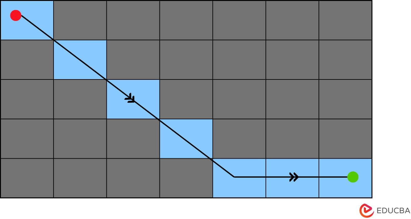
start_state = (0, 0)
goal_state = (4, 6)
path = astar(start_state, goal_state, manhattan_distance, successors)
print("Path:", path)

Output:

Visual:

Advantages of A-star Algorithm

1. Completeness: A* is complete, indicating it will find a solution if one exists, provided that the heuristic function is admissible (never overestimates the actual cost).
2. Optimality: A* is optimal with an admissible heuristic. It guarantees to find the shortest path from the start node to the goal node, ensuring an optimal solution.
3. Efficiency: A* is generally efficient in terms of time complexity compared to uninformed search algorithms like breadth-first search or depth-first search. It focuses its search on the most promising paths, reducing the number of nodes explored.
4. Adaptability: A* is adaptable to various problem domains and environments. It can be applied to graphs, grids, and networks, making it versatile for pathfinding and optimization tasks.
5. Heuristic Guidance: A* uses heuristic information to guide its search process efficiently. By incorporating an admissible heuristic, A* can prioritize nodes more likely to lead to the goal, reducing unnecessary exploration.
6. Memory Efficiency: A* maintains only a small number of nodes in memory at any given time, making it memory-efficient, especially for large-scale problems.
7. Flexible Heuristic Function: A* allows flexibility in the choice of heuristic function. Developers can customize the heuristic function based on domain-specific knowledge, allowing for tailored solutions to specific problem instances.
8. Applications in Real-world Problems: A* has been successfully applied to various real-world problems, including robotics, video games, logistics, network routing, and more, demonstrating its effectiveness and practical utility.

Limitations of A-star Algorithm

1. Memory Usage: A* can consume significant memory, especially in large graphs or grid scenarios. It needs to store information about explored and open nodes and associated costs.
2. Time Complexity: Although A* is generally efficient, its time complexity can increase significantly in scenarios where the number of nodes or edges is large. In worst-case scenarios, A* may perform poorly compared to less sophisticated algorithms.
3. Heuristic Quality Dependency: The efficiency and optimality of A* heavily depend on the quality of the heuristic function used. If the heuristic function is not admissible (overestimates the actual cost) or inconsistent, A* may fail to find the optimal solution or take longer to converge.
4. Admissibility Requirement: A* requires an admissible heuristic function to guarantee optimality. Finding or designing such a heuristic can be challenging in some problem domains. In cases where an admissible heuristic is unavailable, the performance of A* may degrade.
5. Potential for Suboptimal Solutions: In scenarios where the heuristic function is not admissible or the search space is complex, A* may find suboptimal solutions instead of the globally optimal one. It occurs when the algorithm prematurely terminates its search before reaching the optimal solution.
6. Pathological Cases: A* may encounter pathological cases, such as highly symmetric or cyclic graphs, where the search process becomes inefficient or fails to terminate within a reasonable time frame.
7. Difficulty Handling Dynamic Environments: Design A* for static environments where the cost of moving between nodes remains constant. In dynamic environments where the costs change over time or due to external factors, A* may need to be adapted or combined with other techniques to handle such scenarios effectively.
8. No Guarantees for Negative Edge Costs: A* does not guarantee optimal solutions in graphs with negative edge costs. In such cases, algorithms like Dijkstra’s algorithm or Bellman-Ford may be more suitable.

Real-World Applications

1. GPS Navigation Systems: A* calculates the shortest or fastest route between two locations. It helps drivers or users navigate through road networks efficiently, considering traffic conditions, road closures, and real-time data.
2. Robotics and Autonomous Vehicles: A* plays a crucial role in robotics and autonomous vehicles for path planning and navigation. Robots and self-driving cars use A* to plan optimal paths in dynamic environments, avoid obstacles, and reach their destinations safely and efficiently.
3. Video Games: The industry uses A* for NPC (Non-Player Character) pathfinding, enemy AI navigation, and game-level design. It allows developers to create realistic and challenging game environments where characters intelligently navigate complex terrains and obstacles.
4. Logistics and Supply Chain Management: Companies apply A* for route optimization, vehicle routing, and warehouse management. It helps logistics companies minimize transportation costs, reduce delivery times, and improve operational efficiency.
5. Air Traffic Management: Air traffic management systems employ A* for aircraft route planning and scheduling. It assists air traffic controllers in managing air traffic flow, optimizing flight paths, and ensuring safe and efficient operations within airspace.
6. Emergency Response and Disaster Management: A* is used in emergency response and disaster management scenarios to plan evacuation routes, allocate resources, and coordinate rescue operations. It helps responders optimize their efforts and minimize response times during emergencies and natural disasters.
7. Network Routing and Packet Switching: A* is utilized in computer networks to route packets between network nodes. It helps optimize data transmission routes, reduce network congestion, and improve network performance in wired and wireless communication systems.
8. Terrain Analysis and Geographic Information Systems (GIS): GIS applications apply A* for terrain analysis, land use planning, and spatial data processing. It assists urban planners, environmental scientists, and geospatial analysts in analyzing geographic data, locating resources, and planning infrastructure projects.

Conclusion

The A* algorithm widely recognizes its versatility and effectiveness in addressing pathfinding and optimization challenges across various domains. With its capacity to navigate through intricate environments efficiently and ensure optimality in certain conditions, A* has been extensively adopted in real-world scenarios like GPS navigation, robotics, logistics, and video games. While it has limitations, its advantages often outweigh drawbacks, contributing significantly to enhanced efficiency, safety, and decision-making in diverse fields. As technology progresses, A* remains pivotal in tackling complex pathfinding and optimization tasks.

Frequently Asked Questions (FAQs)

Q1. Can A be used in dynamic environments where the cost of moving between nodes changes over time?*

Answer: Design A* primarily for static environments where the cost of moving between nodes remains constant. However, adaptations and extensions of A* exist to handle dynamic environments, such as online variants of A* that dynamically update the heuristic estimates based on changing conditions.

Q2. Is A guaranteed to terminate if a solution exists?*

Answer: A* is guaranteed to terminate and find a solution if one exists in finite graphs or bounded search spaces. However, in infinite graphs or unbounded search spaces, A* may not terminate if the goal node is unreachable or the heuristic function is not admissible.

Q3. How can I choose an appropriate heuristic for my A algorithm?*

Answer: Choosing an appropriate heuristic depends on the specific problem domain and characteristics of the search space. Common heuristics include Manhattan, Euclidean, and Chebyshev distances for grid-based problems and custom heuristics based on domain-specific knowledge.

Recommended Articles

1. Ternary Search
2. Interpolation Search Algorithm
3. Search Algorithms in AI
4. Clustering Algorithms