Updated August 21, 2023
Introduction to YEAR Formula in Excel
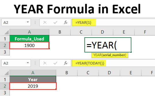
Year Formula in Excel simply returns the year from the selected date cell. And the value we will get obviously in 4 digit year containing the century and year out of that century. The syntax of the Year function considers only the serial number, but we can even select the cell with the date, and this function will extract the same out of it. Feeding the 1 in-Year function will return 1900 as the first year available in MS Office.
Syntax:
An argument in YEAR Formula
- serial_number: Serial Number represents the date.
Explanation
If you are confused about how the serial number represents the date? Then you should understand how data save in Excel. From 1 Jan 1900, excel assigned a serial number to each date. For 1 Jan 1900 one, 2 Jan 1900 two and so on.
For example, if we give serial number 1 in the year formula, it will return 1900 per the logic below.
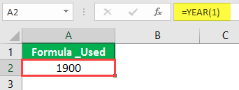
Observe the formula; we just input 1 in the serial number, and it returned 1900, the year related to that date. We will see a few more examples of how to use the YEAR function.
How to Use Excel YEAR Formula in Excel?
Excel YEAR Formula is very simple and easy. Let’s understand how to use the Excel YEAR Formula with a few examples.
Example #1 – YEAR Formula with DATE Function
To know the 4-digit year, we need to input the date’s serial number. But, how can we every time calculate the serial number for a date every day? So, instead of using the serial number, we can use the date formula.
Follow the steps below to get the year from a date using the date formula instead of the serial number.
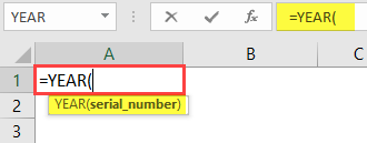
First, start the YEAR Formula as below.
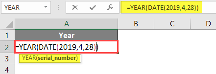
Input the DATE Formula in place of the serial number as below.

We must input the year, month, and day in the DATE Formula.
Press Enter Key.
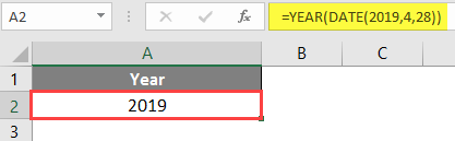
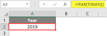
As we have input the Year as 2019 in the date formula, it returns the year as 2019.
Example #2 – Year Formula with TODAY Function
If we want to get the current year details using the Today function, we can easily get it. Follow the below steps.
Start the Year Formula as below.
We need to get today’s 4-digit year number, hence the input TODAY function.
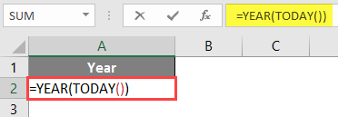
Press Enter after closing the TODAY function. It will return the current year number as below.
Example #3 – Comparing Two Dates
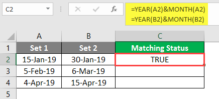
They are comparing two dates, whether they belong to the Same Month and Year. Consider two sets of different dates like the below screenshot.
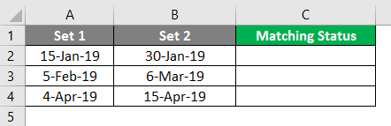
Now with the help of the year and month function, we will check how many days in the same row are related to the same month and year.
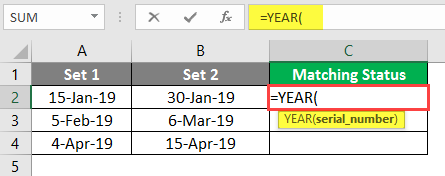
Start the Formula with the YEAR first, as below.
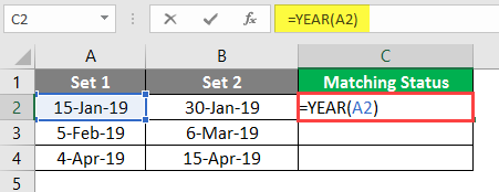
Select the First Date Cell from Set 1.
Now Add & Symbol and add MONTH function for the same cell as below.

Up to now, we have merged the year and month of the first date from set 1. Similarly, do for the first date from set 2 also.
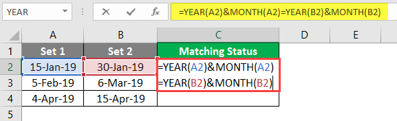
Now it will return if the month and year of both dates are matched. If the year or month anyone criteria is not matched, it will return False.
Drag the same formula to the other cells.
Example #4 – Find the Year is Leap Year or Not
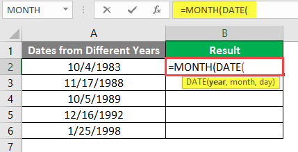
Take a few dates from different years, as shown in the below screenshot.
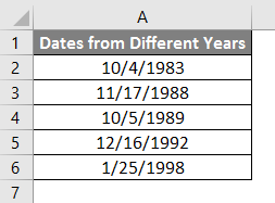
We need to find which date belongs to the leap year from the above data. Follow the below steps to find the leap year using the YEAR function.
Start the Formula with the MONTH Function.
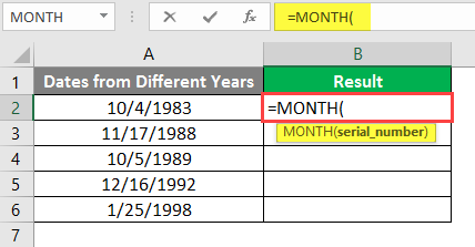
Instead of inputting the serial number, input the DATE function, as shown in the below screenshot.
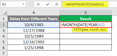
Instead of inputting the year directly, use the YEAR function and choose the cell with the date.
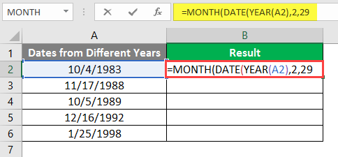
For the “MONTH” argument, input 2, and for the “DAY” argument, input 29.
Close the DATE and MONTH brackets, then input equal to “=” 2 as shown below.
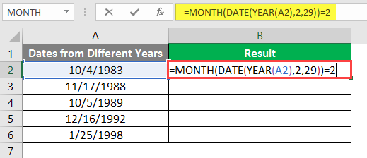
Press Enter Key.

Drag the Same Formula to other cells.
Conclusion
From all the dates, we want to know whether February has 29 days or not for that year; February is the second month, so the formula “Month” function should return 2. It will return 2 only when the Date function is correct; that means if that year February has 28 days, it will scroll to March 1st and return 3, so the result of the Month formula will not match with the number 2.
Whenever February has 29 days, it will return 2, which will match the right-hand side 2 and return “True”.
This is one way; otherwise, we can find it differently, as below.
1. Left-hand side calculates the date after February 28; if it is equal to the right-hand side 29, then it is a leap year.
2. Left-hand side calculates the date before March 1; if it is equal to the right-hand side 29, then it is a leap year.
Things to Remember About YEAR Formula in Excel
- The year formula is helpful when we require the details of a year alone from a large bunch of data.
- Never input the Date directly in the Year function as it will consider it as text and will return the error #NAME as it will consider only as text.
- If you want to use the year function directly, take the help of the Date function and use it, then you will not get any error.
- Another way of using it is to convert the date into number format and use that number in the serial number to get the 4-digit year.
- If you took the year before 1900, you would get the error message #VALUE hence ensure you are using the YEAR function for the years after 1900.
- Ensure the date format is correct because using a value greater than 12 in a month or greater than 31 in the day will throw an error.
Recommended Articles
This is a guide to the YEAR Formula in Excel. Here we discuss How to use the YEAR Formula in Excel, practical examples, and a downloadable Excel template. You can also go through our other suggested articles –