Updated March 13, 2023

Introduction to Time series in R
Time series in R is defined as a series of values, each associated with the timestamp also measured over regular intervals (monthly, daily) like weather forecasting and sales analysis. The R stores the time series data in the time-series object and is created using the ts() function as a base distribution.
Syntax
The Syntax declaration of the Time series function is given below:
<- ts(data, start, end, frequency)
Here data specify values in the time series.
start specifies the first forecast observations in a time series value.
end specifies the last observation value in a time series.
frequency specifies periods of observations (month, quarter, annual).
How Time-series works in R?
R has a powerful inbuilt package to analyze the time series or forecasting. Here it builds a function to take different elements in the process. At last, we should find a better fit for the data. The input data we use here are integer values. Not all data has time values, but their values could be made as time-series data. The data consists of observations over a regular interval of time. It needs several transformations before it is modeled up. The time series has the following elements:
- Trend: It is categorized under the sinusoidal effects means the data either decreases or increases during a long period.
- Seasonality: It’s calendar-related effects. The observed data have to be seasonally adjusted by undergoing true movement in the series. So it undergoes some peaks and decreases in the plot each year.
- Level: It represents a baseline value for the series.
- Noise: An error or irregular variations foreseen.
The most familiar ways of fitting the series are to use either autoregressive, moving average or both. The other way to access is to use Autocovariance and partial autocovariance function, respectively.
Let’s see how time series are forecasted in R
Preparing time series
- Creating an array of data to analyze it. For example, a data frame is given according to the forecasting sales value by quarter, half-yearly or yearly.
y<-c(1.8, 1.1, 3, 3.5, 4.8, 4.2, 5.8, 6.4, 5, 7, 7.4, NA, NA, NA, NA)

data <- data.frame(t=x, cases=y)

data

2.          t cases

3.      1   1   1.8

4.      2   2   1.1

5.      3   3   3.0

6.      4   4   3.5

7.      5   5   4.8

8.      6   6   4.2

9.      7   7   5.8

10.   8   8   6.4

11.   9   9   5.0

12.   10 10   7.0

13.   11 11   7.4

14.   12 12    NA

15.   13 13    NA

16.   14 14    NA

17.   15 15    NA

NA are the values that we need to forecast.
Naïve Forecasting
naiv_ex <- naive(data, h = 12)

summary(naiv_ex)
ARIMA model
Auto.arima()
Decomposition: The time series has multiple patterns, and the process of isolating them is known as decomposition.
Plotting time series
Plot (x)
Note:
In R head () used for older observations, an existing value in the dataset. tail () – gives newer observations. Modified predicted value.
Examples
The code here has been implemented using RStudio and install the necessary packages. Most Importantly forecast library is used to predict future events. And we can take R built-in datasets for performing time series analysis.
Example #1
stockrate <- c(480, 6813, 27466, 49287,
7710, 96820, 96114, 236214,
2088743, 381497, 927251,
1407615, 1972113)
> stockrate.timeseries <- ts(stockrate,start = c(2019,1),frequency = 12)
> print(stockrate.timeseries)
Jan Feb Mar Apr May Jun Jul
2019 480 6813 27466 49287 7710 96820 96114
2020 1972113
Aug Sep Oct Nov Dec
2019 236214 2088743 381497 927251 1407615
2020
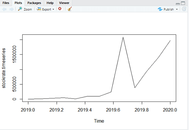
> plot(stockrate.timeseries)
Explanation
The complete Output is shown here, which makes predictions for the stock rate for the year 2019.
Output:
The Time series Plot is given as
Example #2
Demonstrating Multiple Time-series
stockrate <- c(450, 613, 466, 205.7,
571.0, 622.0, 851.4, 621.4,
875.3, 979.7, 927.5,
14.45, 12.23)
> stockrate2 <- c(550, 713, 566, 687.2,
110, 120, 72.4, 814.4,
423.5, 98.7, 741.4,
345.3, 323.2)
> combined.stockrate <- matrix(c(stockrate,stockrate2),nrow = 12)
Warning message:
In matrix(c(stockrate, stockrate2), nrow = 12) :
data length [26] is not a sub-multiple or multiple of the number of rows [12]
> stockrate2 <- c(550, 713, 566, 687.2,
110, 120, 72.4, 814.4,
423.5, 98.7, 741.4,
345.3)
> stockrate <- c(450, 613, 466, 205.7,
571.0, 622.0, 851.4, 621.4,
875.3, 979.7, 927.5,
14.45)
> combined.stockrate <- matrix(c(stockrate,stockrate2),nrow = 12)
> stockrate.timeseries <- ts(combined.stockrate,start = c(2014,1),frequency = 12)
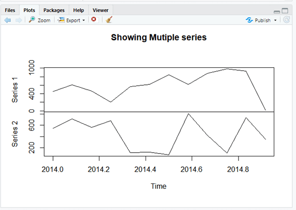
> plot(stockrate.timeseries, main = "Showing Mutiple series")
> print(stockrate.timeseries)
Series 1 Series 2
Jan 2014 450.00 550.0
Feb 2014 613.00 713.0
Mar 2014 466.00 566.0
Apr 2014 205.70 687.2
May 2014 571.00 110.0
Jun 2014 622.00 120.0
Jul 2014 851.40 72.4
Aug 2014 621.40 814.4
Sep 2014 875.30 423.5
Oct 2014 979.70 98.7
Nov 2014 927.50 741.4
Dec 2014 14.45 345.3
Explanation
This shows the time series plot taking two forecasting values.
Output:
Multiple time series Plot is given as
Example #3
data("austres")
> start(austres)
[1] 1971 2
> end(austres)
[1] 1993 2
> sum(is.na(austres))
[1] 0
> summary(austres)
Min. 1st Qu. Median Mean 3rd Qu. Max.
13067 14110 15184 15273 16399 17662
> plot(austres)
> tsdata <- ts(austres, frequency = 12)
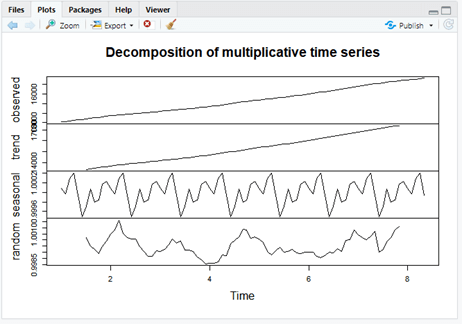
> dcdata <- decompose(tsdata, "multiplicative")
> plot(dcdata)
> head(austres)
Qtr1 Qtr2 Qtr3 Qtr4
1971 13067.3 13130.5 13198.4
1972 13254.2 13303.7 13353.9
> newmodel=auto.arima(austres)
> newmodel
Series: austres
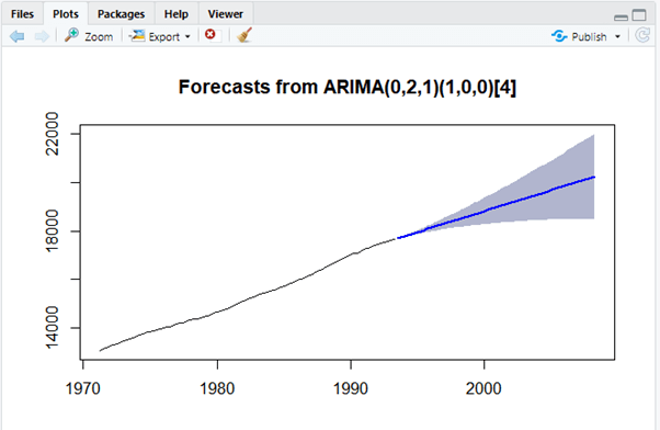
ARIMA(0,2,1)(1,0,0)[4]
Coefficients:
ma1 sar1
-0.6051 0.1921
s.e. 0.0974 0.1075
sigma^2 estimated as 103.7: log likelihood=-322.93
AIC=651.86 AICc=652.15 BIC=659.26
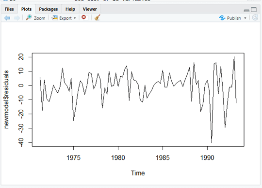
> plot.ts(newmodel$residuals)
> ffcast <- forecast(newmodel, level=c(80), h=5*12)
> plot(ffcast)
// Taking ACF and PACF
acf(ffcast$residuals)
> pacf(ffcast$residuals)
> coef(ffcast)
NULL
predict(ffcast, n.ahead=5, se.fit=TRUE)
forecast(object=ffcast, h=5)
Point Forecast Lo 80 Hi 80
1993 Q3 17704.82 17691.77 17717.87
1993 Q4 17748.00 17725.60 17770.40
1994 Q1 17794.20 17761.83 17826.56
1994 Q2 17835.79 17792.65 17878.92
1994 Q3 17879.09 17822.79 17935.39
Explanation
In the above R code, we will use a dataset austres with information about the sales from the year 1971 to 1993. And Using ARIMA, we have predicted the sales of the year (next five years)2000, which is shown in the plot with the blue indicator.
Plot:
Plotting new model residuals
Forecasting using ARIMA
Conclusion
Therefore, in this article, we covered many details on Time Series in R and also learned the stationary process and many more with the implementation. Time series performs an important statistical technique that collects data points in chronological order.
Recommended Articles
This is a guide to the Time series in R. Here; we discuss How Time-series works in R along with the examples and outputs. You may also have a look at the following articles to learn more –
