Updated May 15, 2023
Excel ROWS Function (Table of Contents)
Introduction to ROWS Function in Excel
Excel is nothing more than a table with rows and columns. Every time we work on Excel, we have to deal with cells. A cell is nothing but intersection rows and columns. While working on cells, we always will come up with a situation where we need to figure out how many ranges of rows we are working on. There comes the Excel ROWS function to your help, allowing you to calculate the number of rows present in an array.
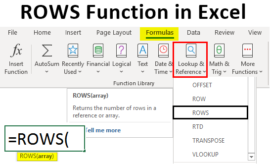
Excel ROWS function is categorized under Lookup & Reference functions section under Formulas in Excel. This means this function can look up the values/numbers or find the references. And that is what the function does itself; it looks up the rows in an array/reference provided and gives the number of those rows as an output. You can see the definition of the function when you navigate your mouse toward the same. Below is the screenshot that makes things look clearer.
Syntax of ROWS Function
The argument of ROWS Function:
Array – This is a required argument that specifies the range of cells used as an argument and function that captures the number of rows for the same.
How to Use ROWS Function in Excel?
With some examples, let’s understand how to use the ROWS Function in Excel.
Example #1 – Calculate the Number of Rows
To check how the Excel ROWS function work, follow the below steps:
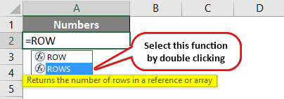
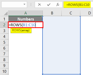
Step 1: In an active Excel sheet, start typing the syntax as =ROW and select the ROWS function by double-clicking from the list of functions that will appear as soon as you start typing the function syntax.
Step 2: As soon as you double click the ROWS function from the list, it will appear inside the cell you are referring to and ask for an argument, i.e. an array for cell reference through which the function can count the number of rows.

Step 3: Now, we need to provide an array of cells as an argument to this function. Put B1:C10 as an array argument to ROWS Function.
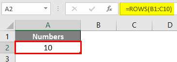
Now, we will figure out what could be the output for this function with B1:C10 as an argument. The array is up to the 10th row of Excel irrespective of a column if you can see. Also, the ROWS function doesn’t figure out column numbers. Therefore, the ideal output should be 10 under cell A1.
Step 4: Complete the formula by adding closing parentheses after an array input argument and press Enter key to see the output.
Example #2 – Calculate the Number of Rows for an Array Constant
ROWS function also works on array constants. Array constants are something that are numbers under curly brackets. Ex. {1;2;3}
Step 1: In cell A2 of the active Excel sheet, start typing =ROW and select the ROWS function from the list that appears.
Step 2: Once the function is selected, use {1;3;5;7;9} as an argument for this function. Separate the array constants with a semicolon instead of a comma. Doing so converts them into individual array constants.

Step 3: Complete the ROWS function with closing parentheses and Press Enter key to see the output.
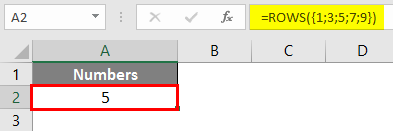
This code considers each constant as a row number and gives the count of all such present in an array. For example, 1 stands for 1st row, 3 for 3rd, and so on. The interesting thing to note down is this example does not include the rows in between. The 2nd, 4th, 6th, and 8th rows are not considered an argument. This is because we used a semicolon as a separator which defines each element of an array as a sole entity.
Example #3 – Count the Table Rows
Suppose we have a table and want to count how many rows the table has acquired. We can do this with the help of the ROWS function as well.
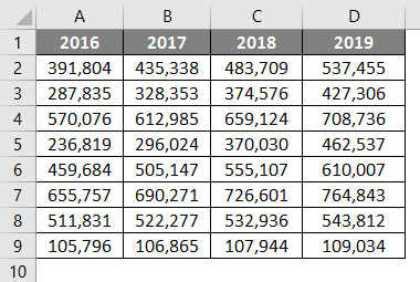
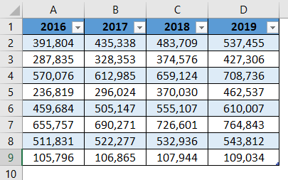
First, we will convert this data into a table. Suppose we have sales data for the past four years, as given below.
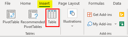
Click on the Insert tab in Excel and click on the Table button to insert a table on given data.
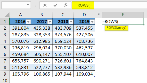
Step 1: In cell F1, start typing the formula =ROWS and select the ROWS function by double-clicking it on the list of suggested functions.
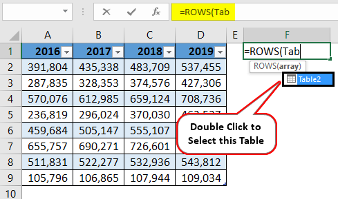
Step 2: Now, it will ask for an array argument to count the number of rows. For that, the type table inside the ROWS function will show the active table present in the system. Double click on it to select.
It will look like the one in the below screenshot. Now we want to check how many rows this table has acquired.
Step 3: Now, it will ask for an array argument to count the number of rows. For that, the type table inside the ROWS function will show the active table present in the system. Double click on it to select.
Step 4: Now close the parentheses so that the formula will be complete, and press the Enter key to see the output.

This will give an output of 8, meaning there are 8 rows in the table. An interesting thing in this example is that whenever we try to capture the rows acquired by a table, the header rows are always neglected from the calculations. See the table; there are 9 rows, including column headers. However, as it is a table, column header rows are neglected.
This is from this article. Let’s wrap things up with some points to be remembered.
Things to Remember
- This function can take an array or any single cell as a reference and returns the number of rows present in that array. If it is a single cell as an argument, it will always return 1 as a row count.
- We can also use array constants or formulas as an argument to this function, which will return the count of rows under array reference.
- Using a table as an argument in this function will return the row count for that table, excluding the column header row.
Recommended Articles
This is a guide to ROWS Function in Excel. Here we discuss How to use the ROWS Function in Excel, practical examples, and a downloadable Excel template. You can also go through our other suggested articles –