Updated June 27, 2023
What is Polynomial in Matlab?
Polynomials are general equations in mathematics that have coefficients and exponent values. In polynomials, exponent values are never negative integers, and it has only one unknown variable. Matlab polynomial are represented as vectors as well as a matrix. Operations such as poly, polyfit, residue, roots, polyval, polyvalm, conv, deconv, polyint, and polyder utilize various functions of polynomials. Various operations on equations use all these functions.
Syntax in Polynomial
Below is the syntax in Polynomial in Matlab:
1. Polyval ( a, 4 )
polyval (function name , variable value)
2. Polyvalm ( a, x )
polyvalm ( function name , variable matrix)
3. R = roots(a)
variable name = roots(function name)
4. Op = polyder(a)
output variable = polyder(input variable name)
5. Op = polyint ( a )
output variable = polyint(input variable name)
6. Op = conv ( a,b)
output variable = conv(polynomial1,polynomial2)
7. Op = dconv ( a,b)
output variable = conv(polynomial1,polynomial2)
How does polynomial work in Matlab?
Polynomial has various forms to evaluate in Matlab. In this, ‘poly’ is used to represent a general polynomial equation. ‘polyeig’ is used to represent Eigenvalue polynomials. ‘polyfit’ is used to represent curve fitting. ‘residue’ is used to represent roots of partial fraction expansion. ‘roots’ used to find roots of polynomials. ‘polyval’ is used to evaluate a polynomial. You can use the tool ‘polyvalm’ to solve problems that involve matrix variables. ‘conv’ is used to find convolution and multiplication of polynomials. ‘deconv’ is used to perform division and deconvolution of polynomials. ‘polyint’ is used for integration and ‘polyder’ is used for differentiation of polynomials.
Steps to Solve Polynomial in Matlab
Step 1: Accept Polynomial Vector.
Step 2: Use Function with Variable Value: Polyval (function Name, Variable Value): Polyvalm ( Function Name, Variable Matrix )
Step 3: Display the Result.
Examples to Implement Polynomial in Matlab
Below are the examples to implement in Polynomial in Matlab:
Example #1
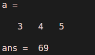
Consider one polynomial a ( x ) = 3 x^2 + 4x + 5
Code:
clear all ;

a = [ 3 4 5 ]
polyval ( a , 4)
Output:
Example #2
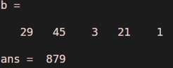
Consider polynomial equation b ( x ) = 2 9 x^4 + 45 x^3 + 3 x^2 + 21 x + 1
Code:
clear all ;

b = [ 29 45 3 21 1 ]
polyval (b , 2)
Output:
Example #3
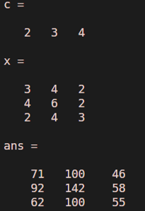
Consider polynomial equation c ( x ) = 2x^2 + 3x + 4
Values of x in the form of the matrix, so,
X = 3 4 2
4 6 2
2 4 3
Code:
clear all ;

c = [ 2 3 4 ]
x = [ 3 4 2 ; 4 6 2 ; 2 4 3 ]
polyvalm (c ,x)
Output:
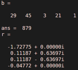
Example #4
Consider one example b ( x ) = 2 9 x^4 + 45 x^3 + 3 x^2 + 21 x + 1
Along with the evaluation of polynomials, we can also find the roots of polynomials:
Code:
clear all ;

b = [29 45 3 21 1]
polyval (b,2)

r = roots(b)
Output:
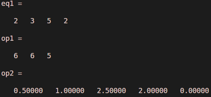
Example #5
Consider polynomial as 2x^3 +3x^2+5x+2
In this example, we will see how to find derivatives and integration of polynomial.
Code:
clear all;

eq1 = [2 3 5 2]
op1 = polyder(eq1)

op2 = polyint(eq1)
Output:
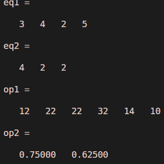
Example #6
Consider two polynomials as eq1= 3x^3 + 4x^2 + 2x + 5 and eq2 = 4 x^2 + 2x + 2
This example illustrates the convolution and deconvolution of two polynomials:
Code:
clear all ;

eq1 = [3 4 2 5]
eq2 = [ 4 2 2]
op1 = conv(eq1,eq2)

op2 = deconv(eq1,eq2)
Output:
Conclusion
In the above sections, we have seen how to evaluate polynomials and how to find the roots of polynomials. Mathematically it is very difficult to solve long polynomials, but in Matlab, we can quickly evaluate equations and perform operations like multiplication, division, convolution, deconvolution, integration, and derivatives.
Recommended Articles
This is a guide to Polynomial in Matlab. Here we discuss an introduction, how polynomial work, and examples to implement with appropriate codes and outputs. You can also go through our other related articles to learn more –
