Updated March 8, 2023

Introduction to Matlab hold on
The following article provides an outline for Matlab hold on. Matlab’s ‘hold’ command determines whether the newly created graphic object will be added to the existing graph or will it replace the existing objects in our graph. The command ‘hold on’ is used to retain our current plot & its axes properties in order to add subsequent graphic commands to our existing graph.
For example, we can add 2 trigonometric waves, sine and cos, to the same graph using the hold on command.
Syntax:
- Command ‘hold on’ is used to retain the plot in current axes. By doing so, the new plot is added to the existing axes without making any changes to the existing plot.
- Command ‘hold off’ is used to change the hold on state back to off.
Examples of Matlab hold on
Let us see how to add a new plot to the existing axes in Matlab using the ‘hold on’ command.
Example #1
In this example, we will use the ‘hold on’ command to add 2 plots to a single graph. We will plot 2 different logarithmic functions in one graph for our 1st example.
The steps to be followed for this example are:
- Initialize the 1st function to be plotted.
- Use the plot method to display the 1st function.
- Use the ‘hold on’ command to ensure that the plot of the next function is added to this existing graph.
- Initialize the 2nd function to be plotted.
- Use the plot method to display the 2nd function.
- Use the ‘hold off’ command to ensure that the next plot, if any, is added as a new graph.
Code:
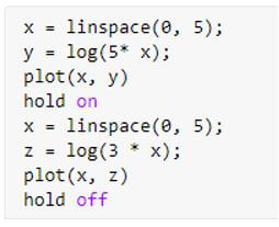
x = linspace (0, 5);
y = log (5* x);
[Initializing the 1st logarithmic function]plot (x, y)
[Using the plot method to display the figure]hold on
x = linspace (0, 5);
z = log (3 * x);
[Initializing the 2nd logarithmic function]plot(x, z)
[Using the plot method to display the figure]hold off
[Using the ‘hold off’ command to ensure that the next plot, if any, is added as a new graph]This is how our input and output will look like in the Matlab command window.
Input:
Output:
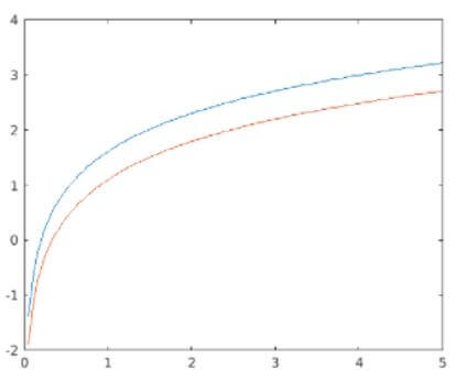
As we can see in the output, we have obtained 2 logarithmic functions in the same graph as expected by us.
Example #2
In this example, we will use the ‘hold on’ command to add 2 different exponential functions in one graph.
The steps to be followed for this example are:
- Initialize the 1st function to be plotted.
- Use the plot method to display the 1st function.
- Use the ‘hold on’ command to ensure that the plot of the next function is added to this existing graph.
- Initialize the 2nd function to be plotted.
- Use the plot method to display the 2nd function.
- Use the ‘hold off’ command to ensure that the next plot, if any, is added as a new graph.
Code:
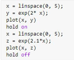
x = linspace(0, 5);
y = exp(2* x);
[Initializing 1st exponential function]plot(x, y)
[Using the plot method to display the figure]hold on
x = linspace(0, 5);
z = exp(2.1 * x);
[Initializing 2nd exponential function]plot(x, z)
[Using the plot method to display the figure]hold off
[Using the ‘hold off’ command to ensure that the next plot, if any, is added as a new graph]This is how our input and output will look like in the Matlab command window.
Input:
Output:
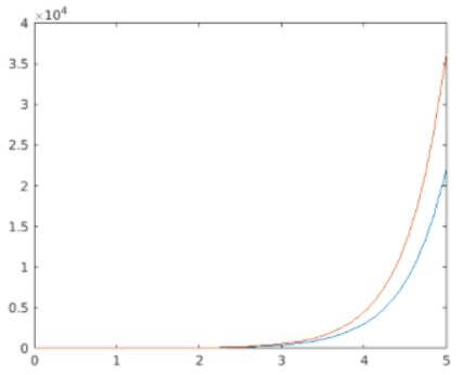
As we can see in the output, we have obtained 2 exponential functions in the same graph as expected by us.
In the above 2 examples, we saw how to add 2 functions to a single graph. We can also use the same ‘hold on’ command to add more than 2 functions also. Next, we will see how to add 3 functions to the same graph.
Example #3
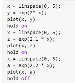
In this example, we will use the ‘hold on’ command to add 3 plots to a single graph. We will plot 3 different exponential functions in one graph for this example.
The steps to be followed for this example are:
- Initialize the 1st function to be plotted.
- Use the plot method to display the 1st function.
- Use the ‘hold on’ command to ensure that the next plot is added to this existing graph.
- Initialize the 2nd function to be plotted.
- Use the plot method to display the 2nd function.
- Use the ‘hold on’ command to ensure that the next plot is added to this existing graph.
- Initialize the 3rd function to be plotted.
- Use the plot method to display the 3rd function.
- Use the ‘hold off’ command to ensure that the next plot, if any, is added as a new graph.
Code:
x = linspace(0, 5);
y = exp(2* x);
[Initializing 1st exponential function]plot(x, y)
[Using the plot method to display the figure]hold on
x = linspace(0, 5);
z = exp(2.1 * x);
[Initializing 2nd exponential function]plot(x, z)
[Using the plot method to display the figure]hold on
x = linspace(0, 5);
a = exp(2.2 * x);
[Initializing 3rd exponential function]plot(x, a)
[Using the plot method to display the figure]hold off
[Using the ‘hold off’ command to ensure that the next plot, if any, is added as a new graph]This is how our input and output will look like in the Matlab command window:
Input:
Output:
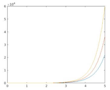
As we can see in the output, we have obtained 3 exponential functions in the same graph as expected by us.
Conclusion
Matlab’s ‘hold on’ command is used to add more than 1 graphic object to the same figure. This command is used to retain our current plot & its axes properties in order to add subsequent graphic commands to our existing graph.
Recommended Articles
This is a guide to Matlab hold on. Here we discuss the introduction to Matlab hold on along with examples for better understanding. You may also have a look at the following articles to learn more –
