Updated April 29, 2023
INT in Excel
INT in Excel is a very simple function used to convert any number into an integer value. Integer values are any number that is a whole number but can be a positive or negative number. Int function can consider any number, whether it is a decimal, fraction, or square root value, but in the end, we will be getting a whole number out of it.
INT Formula in Excel:
Below is the INT Formula in Excel.
where
Number or Expression – It is the number you want to round down to the nearest integer.
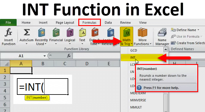
How to Use INT Function in Excel?
INT function in Excel is very simple and easy to use. Let us understand the working of the INT function in Excel by some INT Formula examples. INT function can be used as a worksheet function and VBA function.
Example #1
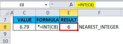
The below-mentioned table contains a value in cell “C8”, i.e. 6.79, which is a positive number; I need to find out the nearest integer for 6.79 using the INT function in Excel.
Select the cell “E8,” where the INT function needs to be applied.

Click the insert function button (fx) under the formula toolbar; a dialog box will appear, type the keyword “INT” in the search for a function box, INT function will appear in the Select a function box. Double-click on the INT function.
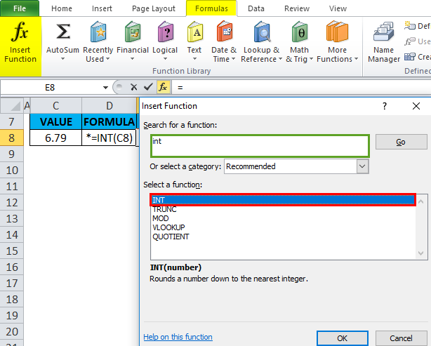
A dialog box appears where arguments (number) for the INT function need to be filled or entered.
i.e. =INT(C8).

It removes the decimal from the number and returns the integer part of the number, i.e. 6.
Example #2
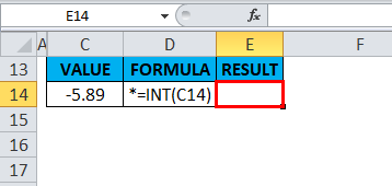
The below-mentioned table contains a value in cell “C14”, i.e. -5.89, which is a negative number; I need to find out the nearest integer for -5.89 using the INT function in Excel. Select cell E14, where the INT function needs to be applied.
Click the insert function button (fx) under the formula toolbar; a dialog box will appear, type the keyword “INT” in the search for a function box, INT function will appear in the Select a function box. Double-click on the INT function.
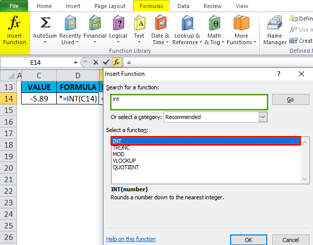
A dialog box appears where arguments (number) for the INT function need to be filled or entered.
i.e. =INT(C14)
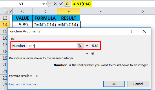
It removes the decimal from the number and returns the integer part of the number, i.e. -6.
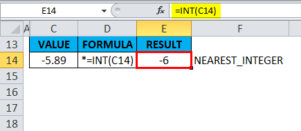
When the INT function is applied to a negative number, it rounds it down. i.e. It returns the number lower than the given number (More negative value).
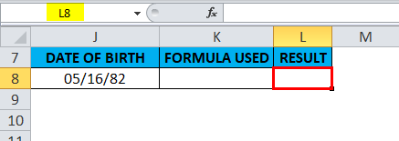
Example #3
In the below mention example, I have the date of birth ( 16th May 1982) in cell “J8” I need to calculate the age in cell “L8” using the INT function in Excel.
Before the INT function in Excel, let’s know about the YEARFRAC function; the YEARFRAC function returns a decimal value representing fractional years between two dates. I.e. Syntax is =YEARFRAC (start_date, end_date, [basis]). It returns the number of days between 2 dates as a year.
Here the INT function is integrated with the YEARFRAC function in cell “L8”.
YEARFRAC formula takes the date of birth and the current date (given by the TODAY function) and returns the output value as age in years.
i.e. =INT(YEARFRAC(J8,TODAY()))
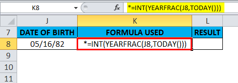
It returns the output value i.e. 36 years.

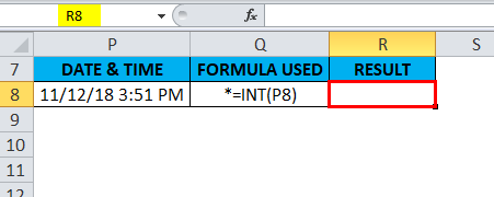
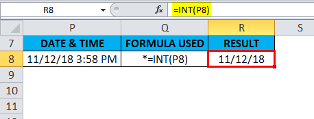
Example #4
Usually, Excel stores the date value as a number, considering the date as an integer and the time as a decimal portion. If a cell contains a date and time as a combined value, you can only extract the date value using the INT function in Excel. Cell “P8” contains the date and time as a combined value. Here I need to extract the date value in cell “R8.”
Select the cell R8 where the INT function needs to be applied.
Click the insert function button (fx) under the formula toolbar; a dialog box will appear, type the keyword “INT” in the search for a function box; the INT function will appear in select a function box. Double-click on the INT function.
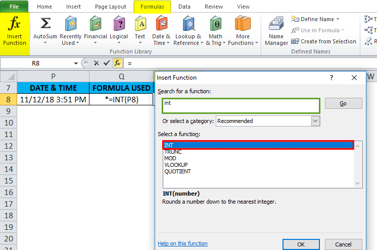
A dialog box appears where arguments (number) for the INT function need to be filled or entered.
i.e. =INT(P8)
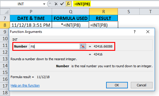
It removes a decimal portion from the date & time value and returns only the date portion as a number, where we need to discard the fraction value by formatting in the output value.
i.e. 11/12/18
Example #5
The below-mentioned table contains a value less than 1 in cell “H13”, i.e. 0.70, which is a positive number; I need to find out the nearest integer for decimal value, i.e. 0.70, using the INT function in Excel. Select cell I13 where the INT function needs to be applied.

Click the insert function button (fx) under the formula toolbar; a dialog box will appear, type the keyword “INT” in the search for a function box, INT function will appear in the Select a function box. Double-click on the INT function.

A dialog box appears where arguments (number) for the INT function need to be filled or entered.
i.e. =INT(H13)

Here, it removes the decimal from the number and returns the integer part of the number, i.e. 0

Things to Remember
- In the INT function, Positive numbers are rounded toward 0, while negative numbers are rounded away from 0. E.G. =INT(2.5) returns 2 and =INT(-2.5) returns -3.
- Both INT() and TRUNC() functions are similar when applied to positive numbers; both can convert a value to its integer portion.
- If any wrong type of argument is entered in the function’s syntax, it results in #VALUE! Error.
- If the referred cell is not a valid or invalid reference in the INT function, it will return or result in #REF! Error.
- #NAME? Error occurs when Excel does not recognize specific text in the formula of the INT function.
Recommended Articles
This has been a guide to INT Function in Excel. Here we discuss the INT Formula in Excel and how to use the INT function in Excel, along with practical examples and downloadable Excel templates. You can also go through our other suggested articles –