Updated June 29, 2023
Introduction to Boxplot in Matlab
The boxplot function is used to represent data graphically concerning the box. It creates a graph of the Boxplot. Depending upon the database and input number of box representations is variable. If only one row or column of data is available in the input Boxplot function will give only one box. And if data is available in the form of a matrix or a number of rows as well as columns, then the boxplot function will give a number of boxes concerning the number of columns. In Boxplot always, we can see one mark in the middle, representing the median of all input data. The bottom side of the box shows a twenty-five percent database proportion the topside or edge shows a seventy-five percent database proportion.
Syntax:
Boxplot (var1)
Boxplot (var1,var2)
Boxplot ( user-defined parameters)
How does Boxplot Calculate in Matlab?
Let us discuss the steps to calculate Boxplot.
Step 1: Accept database (load command)
Step 2: Sort the data in descending or ascending order
Step 3: Find the median of all the values
Step 4: Mark on the rough line
Step 5: Create three quartiles on a rough line
Step 6: Draw a horizontal line by joining quartiles
Step 7: Display the final plot
Examples of Boxplot in Matlab
Given below are the examples of Boxplot in Matlab:
Example #1
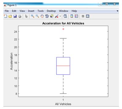
Consider one example of an inbuilt database of cars. ( “car small” ) in this database acceleration, origin all this information is available. We can create a Boxplot by assigning any value parameter from the above options. Let us consider the acceleration parameter. There are 100 acceleration entries so that we can plot an acceleration graph concerning all vehicles. In this case, we are considering only one parameter, acceleration, to get only one box in the output.
Code:
clear all ;

clc ;

load carsmall

boxplot (Acceleration)

xlabel ( 'All Vehicles' )

ylabel ( 'Acceleration' )

title ( 'Acceleration for All Vehicles' )
Work space:
(Database values of acceleration, for example, 1, example 2, and example 3)
12 11.50 11 12 10.50 10 9 8.50 10 8.50 17.50 11.50 11 10.50 11 10 8 8 9.50 10 15 15.50 15.50 16 14.50 20.50 17.50 14.50 17.50 12.50 15 14 15 13.50 18.50 15.50 16.90 14.90 17.70 15.30 13 13 13.90 12.80 15.40 14.50 17.60 17.60 22.20 22.10 14.20 17.40 17.70 21 16.20 17.80 12.20 17 16.40 13.60 15.70 13.20 21.90 15.50 16.70 12.10 12 15 14 19.60 18.60 18 16.20 16 18 16.40 20.50 15.30 18.20 17.60 14.70 17.30 14.50 14.50 16.90 15 15.70 16.20 16.40 17 14.50 14.70 13.90 17.30 15.60 24.60 11.60 18.60 19.40
Output:
Example #2
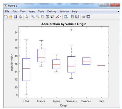
Now let us consider we wish to plot concerning two parameters, so if there is more than one parameter, we will get multiple boxes at the output. In this example, we consider two parameters acceleration and origin. At the output, we can see separate boxes for each origin (country – France, USA, Japan, Germany, Sweden, and Italy).
Code:
clear all ;

clc ;

load carsmall

boxplot (Acceleration ,Origin)

title ( 'Acceleration by Vehicle Origin' )

xlabel ( 'Origin')

ylabel ( 'Acceleration' )
Output:
Example #3
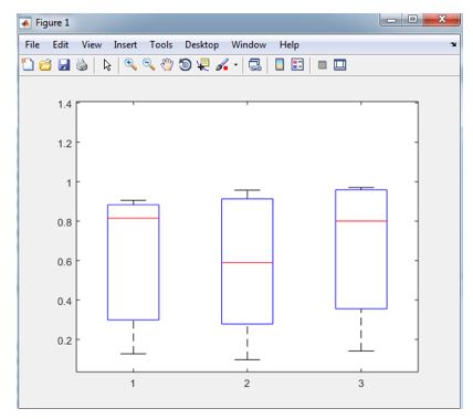
In the third example, here we use two parameters that are not inbuilt. Here we use user-defined parameters. To create a parameter, here default range is assigned then the rand operation is used to create the first parameter. And the second parameter is created by using the repmat function. Repmat function is used for array manipulations, so three arrays or vectors are used in the second parameter. These two user-defined parameters are var 1 and var 2.
Code:
clear all ;

clc ;

rng ( 'default' )

v1 = rand (3 , 1) ;

v2 = rand (6 , 1) ;

v3 = rand (9 ,1) ;

var1 = [ v1 ; v2 ; v3]
v4 = repmat ({ '1' } ,3,1) ;

v5 = repmat ({ '2' } ,6,1) ;

v6 = repmat ({ '3' } ,9,1) ;

var2 = [ v 4 ; v 5 ; v 6 ] ;

boxplot ( var1 ,var2)
Command window:
var1 =
0.8147 0.9058 0.1270 0.9134 0.6324 0.0975 0.2785 0.5469 0.9575 0.9649 0.1576 0.9706 0.9572 0.4854 0.8003 0.1419 0.4218 0.9157
Output:
Conclusion
In this article, we have seen how to create a box plot using the database. While creating a box plot, we can change box colors, box outline size, median style, plot size, plot style, notch status, etc. By using a box plot, we can represent the database very efficiently.
Recommended Articles
This has been a guide to Boxplot in Matlab. Here we discuss the introduction, examples, and how Boxplot calculates in Matlab. You may also have a look at the following articles to learn more –
