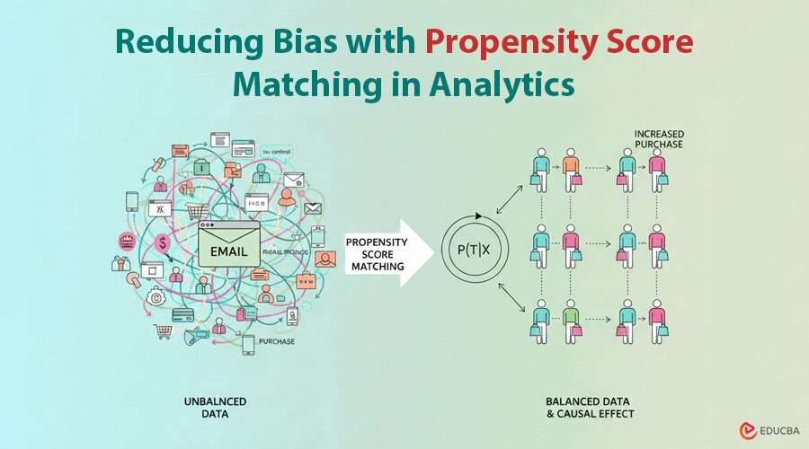
The Need for Causal Inference in Observational Data
In data science, determining whether an intervention caused a change in an outcome goes beyond correlation; this is the essence of causal inference. Observational data, unlike randomized experiments, often suffer from confounding, where certain variables affect both treatment assignment and outcomes. For instance, in marketing, loyal customers may be more likely to receive a promotion and more likely to purchase regardless. Comparing their purchase rates naively to those of other customers would overstate the promotion’s impact. To draw valid causal conclusions, data scientists need methods to adjust for these confounders and approximate a fair comparison between groups. This is where propensity scores become a crucial tool.
What is a Propensity Score?
A propensity score shows how likely a unit (e.g., a customer) is to receive a treatment given its observed characteristics. Formally, if W indicates treatment and X represents covariates, the propensity score for an individual with features X=x is:
Typically, propensity scores are estimated using logistic regression or other classification methods to predict treatment assignment from covariates. The key intuition is that two individuals with the same propensity score have similar probabilities of receiving treatment, given their observed characteristics. Therefore, researchers can more credibly attribute differences in outcomes between them to the treatment itself.
Example Scenario: Email Campaign Effect on Purchases
Imagine an online retailer ran a promotional email campaign to encourage purchases. Unlike a randomized experiment, the marketing team targeted specific customers, for instance, those who had shopped recently or spent more in the past, while others did not receive the email. Our goal is to estimate the causal effect of the email on purchase behavior: did the email actually increase the purchase rate, or were other factors at play?
Observational Challenges
This estimation is challenging because the treated customers (email recipients) differ systematically from the control group (non-recipients). Recent shoppers and high spenders are more likely to be targeted, indicating that pre-existing differences, such as recency of purchase and spending history, act as confounders. Ignoring these can bias the campaign’s estimated effect.
Dataset Overview
Suppose we have data on a cohort of customers, including:
- Treatment: Whether they received the promo email (Yes/No)
- Outcome: Whether they purchased in the subsequent period
- Covariates:
- Recency: Months since last purchase
- History: Total spending in the past year
- Newbie: Whether the customer has been new in the past year
- Channel: Primary channel of past purchases (e.g., web, phone)
In our dataset:
- 35% of customers were treated (received the email)
- 65% were controls (did not receive the email)
Covariate Differences Between Groups
| Covariate | Treated (Email) | Control (No Email) |
| Recency (months since last purchase) | 4.4 | 6.7 |
| History (past year spending $) | 765 | 490 |
| Newbie (% new customers) | 9.8% | 20.7% |
As expected, the treated group consists of more active and valuable customers:
- They purchased more recently (4.4 months vs. 6.7 months)
- They spent more in the past year ($765 vs. $490)
- They are less likely to be new customers (9.8% vs. 20.7%)
These differences indicate substantial confounding.
Naive Outcome Comparison
If we compute the purchase rate without adjustment:
- Treated customers: 6% purchased
- Control customers: 0% purchased
This gives a raw difference of ~6.6 percentage points, suggesting a large effect. However, much of this difference may be due to pre-existing characteristics. Treated customers were inherently more likely to buy because they were more engaged to begin with. Without adjusting for confounders, we risk overestimating the true effect of the email campaign.
Propensity Score Matching to Adjust for Confounders
PSM is a common method for adjusting for confounders in observational studies and approximating a causal comparison. The key idea is to pair each treated customer with one or more untreated customers with similar propensity scores, i.e., similar probabilities of receiving the treatment given observed covariates. This process creates a matched sample in which the distribution of covariates is more balanced across the treated and control groups.
Matching on the propensity score balances multiple covariates at once, making the treatment and control groups comparable. Essentially, propensity score matching simulates a randomized experiment after the fact, ensuring that the treated and control groups are similar with respect to observed characteristics.
How Matching Works in the Email Campaign Example?
For the email campaign scenario:
- Propensity scores were estimated using logistic regression. The model predicted the probability of receiving the email based on customer covariates:
- Recency (months since last purchase)
- History (past year spending)
- Newbie status (new customer or not)
- Channel (primary purchase channel)
- Customers who recently purchased or spent more in the past had higher propensity scores, indicating a higher likelihood of being targeted by the campaign. In contrast, infrequent or low-spending customers had lower propensity scores.
- The analysis employed one-to-one nearest-neighbor matching, pairing each treated customer with the control customer whose propensity score was closest. The analysis excluded customers without suitable matches (e.g., very high-spending individuals with no comparable controls). Using a subset of the control group, it matched most treated customers.
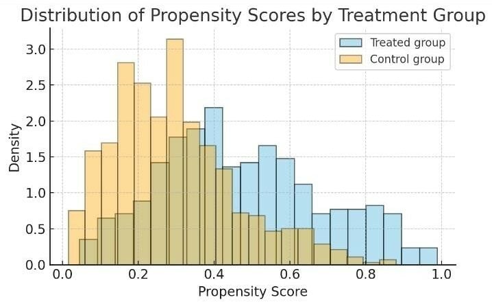
Distribution of propensity scores for customers who received the promotional email (treated) vs those who did not (control).
Checking Covariate Balance
After matching, it is important to verify that the treated and control groups are more balanced with respect to observed covariates. The following table summarizes covariate values before and after matching:
| Covariate | Treated (Before) | Control (Before) | Treated (Matched) | Control (Matched) |
| Recency (months) | 4.4 | 6.7 | 4.4 | 4.9 |
| History ($) | 765 | 490 | 765 | 587 |
| Newbie (%) | 9.8% | 20.7% | 9.8% | 8.7% |
Interpretation
- Recency: The average recency for controls decreased from 6.7 months to 4.9 months after matching, closer to the treated group value of 4.4 months.
- Newbie Percentage: The gap between groups virtually disappeared, with both treated and matched controls around 9%.
- History (Past Spend): The treated group still had slightly higher spending ($765 vs $587), indicating a residual imbalance, likely due to limited overlap: a few control customers had as high spending as treated customers.
Overall, propensity score matching substantially improved covariate balance, making the treated and control groups more comparable and reducing bias in the estimated effect of the email campaign.
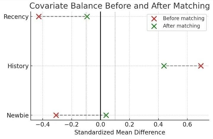
Covariate comparison before and after propensity score matching.
Estimating the Treatment Effect
Using the matched sample of comparable customers, analysts can estimate the treatment effect more credibly. In this example:
- Purchase rate among matched treated customers: 10.6%
- Purchase rate among matched control customers: 5.6%
This results in an estimated lift of approximately 5 percentage points attributable to the email campaign. This effect is lower than the naive 6.6-point difference observed before matching because confounding factors inflated the earlier result.
After matching, the analysis compares each emailed customer to a similar customer who did not receive the email. Therefore, the difference in outcomes is more likely due to the email itself rather than pre-existing purchase propensities. Propensity score matching reduces bias in the estimate by controlling for observed confounders. The analysis indicates that the promotional email had a positive effect on purchases, though the impact is more modest than a raw comparison would suggest.
Limitations of Naive Propensity Score Methods
While propensity score methods are a powerful tool for estimating causal effects in observational studies, they come with important limitations and assumptions.
#1. Only Adjust for Observed Confounders
Propensity score methods adjust only for observed variables included in the model. Any unmeasured factors that influence both treatment and outcome, such as customer satisfaction or offline purchasing behavior, can still bias the results. This means correlation does not imply causation unless the analysis accounts for all major confounders.
#2. Overlap (Common Support) Requirement
For these methods to work reliably, each treated unit should have a comparable control unit with a similar propensity score, and vice versa. If some treated customers are unique (for example, very high propensity with no similar controls), analysts cannot reliably estimate their effect. During matching, analysts may exclude unique units, which limits the results to matchable customers. Lack of overlap can also increase uncertainty in other propensity score approaches that use weighting.
#3. Sensitivity to Model Specification
Propensity scores depend on correctly modeling the relationship between covariates and treatment. Leaving out an important variable or misrepresenting a relationship (e.g., treating a non-linear effect as linear) can leave residual confounding. Choosing the appropriate covariates requires care; too few can introduce bias, too many can add noise or worsen balance. Checking balance diagnostics is essential.
#4. Not a Guarantee of Unbiased Estimates
Propensity scores aim to emulate a randomized experiment, but this is possible only under the assumption of “no unmeasured confounders” (conditional ignorability). Even after matching, hidden bias may persist. Therefore, interpret the results as associational estimates rather than definitive proof of causality, and conduct sensitivity analyses whenever possible.
Key Takeaway:
Propensity score methods reduce bias from observed confounders but cannot fully eliminate it. Be cautious when making causal claims from observational data.
Final Thoughts
Propensity score matching is a practical technique for estimating causal effects in observational studies. It adjusts for known confounders and improves covariate balance, providing a more credible estimate than a naive comparison. Although it accounts only for observable factors and has limitations, it underscores the importance of controlling for confounders in causal analysis. Propensity scores are one tool among many in causal inference. Methods like difference-in-differences, instrumental variables, and regression discontinuity can complement or address their limitations. Advanced approaches, such as doubly robust estimators and Bayesian methods, further refine estimates. Thoughtful use of propensity scores enables more reliable inference about causal effects from observational data.
Author Bio: Dharmateja Priyadarshi Uddandarao

Dharmateja Priyadarshi Uddandarao is an accomplished data scientist and statistician, recognized for integrating advanced statistical methods with practical economic applications. He has led projects at leading technology companies, including Capital One and Amazon, applying complex analytical techniques to address real-world challenges. He currently serves as a Senior Data Scientist–Statistician at Amazon.
Recommended Articles
We hope this guide to propensity scores enhances your understanding of causal inference. Explore these recommended articles for more insights and practical strategies.
