Executive Summary

Genetic matching is a covariate-balancing approach that uses an evolutionary (genetic) search to optimize matches between treated and control groups. Unlike standard matching techniques, genetic matching searches for covariate weights that produce the strongest balance after nearest-neighbor matching. In product experimentation workflows especially A/B-like tests with eligibility gates, triggered analysis, partial rollouts, noncompliance, or exposure filtering pre-balancing matters. Comparing only users who actually received an experience can reintroduce confounding and model dependence. This article demonstrates how to apply genetic matching for causal inference in a product reviews engine experiment, providing a step-by-step guide to:

Defining a causal estimand.
Selecting pre-treatment covariates (e.g., user tenure, prior purchase count, review frequency, product category, device, geography).
Configuring the genetic matching algorithm (distance metric, balance objective, calipers, replacement options).
Conducting matching as a design-stage preprocessing step.
Verifying balance with diagnostics such as standardized mean differences (SMDs), variance ratios, and overlap assessments.

Sample sizes in tables are illustrative; numeric values demonstrate reporting style rather than reflecting actual Amazon data.

The Pre-Balancing Problem in Product Experiments

In an ideal online-controlled experiment, randomization makes the treatment and control groups comparable “by design,” which is why the A/B test is considered a gold-standard causal tool in product development. In real experimentation platforms, however, the causal question teams often want to answer shifts quietly. You might assign users to variant B, but only some users experience B due to conditions such as: model availability by locale, device-specific rendering, category eligibility (e.g., only SKUs with enough reviews), caching fallbacks, or gradual ramp constraints. In practice, these are precisely the kinds of “trustworthiness” pitfalls that large-scale experimentation literature warns about: the theory is simple, but the production details are not. This is where triggered analysis comes into play.

Triggering (also called exposure filtering) focuses analysis on users who could plausibly be affected by the change, thereby materially improving sensitivity. Triggering can be a double-edged sword: if you define the triggered subset by post-assignment behavior (e.g., “users who clicked the reviews tab”), you break the randomized comparison and turn the analysis into disguised observational data. Pre-balancing is a design-stage response to this risk. The core idea is to separate study design (how you construct comparable groups) from outcome analysis (how you estimate effects), and to document balance before looking at outcome differences. Matching is one of the most widely used “nonparametric preprocessing” tools for this purpose because it forces you to confront comparability (overlap) directly rather than hoping a regression model will fix it after the fact.

Understanding Genetic Matching for Causal Inference

Classic nearest-neighbor matching needs a way to decide what “closest” means in a multi-covariate space. If you choose a distance that weights the wrong covariates or weights them inappropriately, you can end up with matches that look close numerically but are imbalanced on the variables that most strongly drive outcomes. Genetic matching addresses this failure mode by learning the distance metric itself.

At a Conceptual Level:

You pick the covariates you want to balance (the “balance targets”).
The algorithm proposes a set of weights (scaling factors) for those covariates and constructs a weighted multivariate distance for matching.
It matches treated and control units using that distance, then scores the result according to a balance criterion.
A genetic (evolutionary) optimizer iterates until balance stops improving.

In its canonical form, genetic matching functions as a general multivariate method, with propensity-score matching and Mahalanobis-distance matching as special cases. In practice, researchers use GenMatch() to learn optimal weights and Match() to perform nearest-neighbor matching with those weights.

Key Advantages in Product Analytics:

Directly optimizes balance rather than relying on propensity-score modeling.
It provides diagnostics to confirm that the matching process achieves balance.

How Genetic Matching Works in Practice?

Most production discussions of matching get stuck at “choose a distance, match, compute an effect.” Genetic matching forces you to be explicit about the design knobs you must set. Many of these are directly exposed in mainstream R tooling (either through the Matching package itself or through wrappers like MatchIt).

1. Distance Metric and Covariate Roles

In standard implementations, genetic matching uses nearest-neighbor matching and computes distances with a generalized (weighted) Mahalanobis metric, where the weights indicate each covariate’s importance. When used through matchit(method = “genetic”), covariates can play multiple roles: (i) variables whose balance is optimized, (ii) variables that enter the distance used for matching, and (iii) variables used to estimate a propensity score if a propensity-score distance is part of the procedure.

2. Balance Objective (“what does the optimizer try to improve?”)

According to the GenMatch() documentation, the method assesses balance with univariate tests, paired t-tests for dichotomous variables, and the Kolmogorov–Smirnov test for multinomial and continuous variables. Users can also select a loss function that aggregates imbalance across covariates. In the MatchIt genetic matching wrapper, the default optimization criterion focuses on covariate balance and typically uses the smallest p-value across balance tests. The algorithm uses this value as a search objective, not as a confirmatory hypothesis test.

3. Covariate Types and Categorical Handling

In product review experimentation, high-cardinality categorical features (product category, geography) are unavoidable and often more predictive than continuous demographics. In matching practice, common strategies include:

One-hot encoding of category indicators (for balance optimization and SMD reporting) with care to avoid ultra-sparse levels.
Exact matching on a small number of high-level categorical partitions (e.g., device family, country group) when violations would be substantively unacceptable.
Calipers that prevent matches across “too far” distances on selected variables (often a propensity-score distance, or critical continuous covariates).

4. Calipers

GenMatch() exposes a caliper argument, and MatchIt’s wrapper explains an important engineering constraint. When you specify calipers in genetic matching, the algorithm incorporates those variables into the matching set used to build the distance matrix because the underlying system operates that way.

5. Replacement vs. No Replacement

You can run genetic matching with or without replacement. Using replacement often improves match quality when the control pool is thin in certain covariate regions. Still, it can reduce the effective sample size and requires inference methods that account for the induced dependence.

6. Computation and Parallelism

Genetic matching is computationally more intensive than “one-shot” matching because each candidate weight set requires rematching and rebalancing. The GenMatch() documentation explicitly supports parallel computation via a cluster option. The Matching package paper also highlights performance engineering details (C++ implementation, BLAS usage, parallelized genetic algorithm), which are relevant to real product datasets.

Applying Genetic Matching for Causal Inference in a Product Reviews Experiment

Consider a realistic product reviews engine change:

Treatment: A new review-ranking algorithm (“Most Relevant Reviews”) that reorders review display using a helpfulness model and user context.
Control: The legacy ranking (“Top Reviews”) is based primarily on helpfulness votes and recency.
Outcome (choose one consistent with your product): purchase conversion within a fixed attribution window after product-page session; or add-to-cart rate; or “helpful vote” engagement. (The exact outcome is unspecified in the prompt; you should define it in advance.)
Unit of analysis: user-level (recommended for independence), defined at first eligible product-page exposure during the experiment window. (Experiment duration and windowing are unspecified.)

Now the twist that motivates matching: the new ranking service is only available for certain product categories and locales, and it sometimes falls back to the control ranking on older app versions. So if you analyze “users who actually saw the new ranking at least once” versus “users who did not,” you are no longer guaranteed a randomized contrast. Triggered analysis fits this scenario well, but you can easily get it wrong if you do not define the triggering set symmetrically or use proper counterfactual logging.

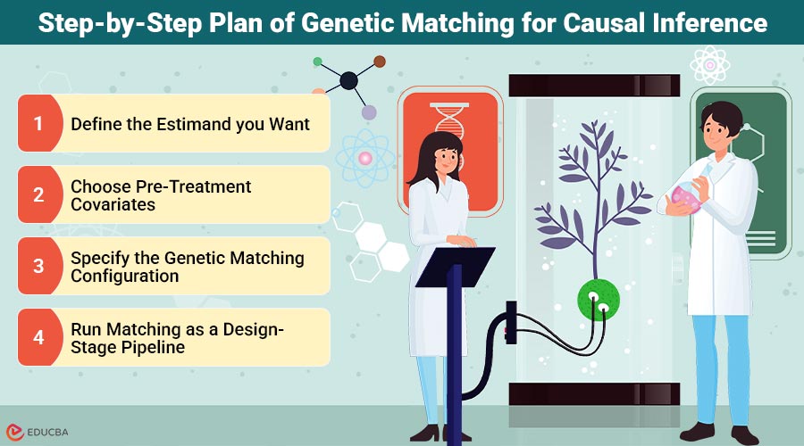
Step-by-Step Plan of Genetic Matching for Causal Inference

1. Define the Estimand you Want

If you keep the analysis at the assignment level, you estimate an intent-to-treat effect and do not need matching. But if your business question is closer to “what is the effect of actually receiving the new ranking,” you are aiming at an exposure-based estimand (often interpreted as an ATT-style estimand for the exposed group). Make that choice explicit because matching changes who you are learning about.

2. Choose Pre-Treatment Covariates

Select covariates measured strictly before exposure/trigger:

User tenure: time since account creation (or first purchase), capturing lifecycle stage.
Prior purchase count: prior orders over a lookback window, capturing demand intensity and familiarity.
Review frequency: propensity to read/write/rely on reviews (e.g., reviews written, helpful votes cast, review panel opens).
Product category: category mix of recent browsing or the category of the first eligible exposure (use coarse groups to prevent sparsity).
Device: web vs. mobile app; OS family.
Geography: country/region (often strongly correlated with product assortment, shipping, and language).

This covariate set is not just a statistical checklist; it reflects plausible confounders in an exposure-based comparison because they influence both (i) eligibility/exposure to the new ranking and (ii) conversion and engagement behaviors.

3. Specify the Genetic Matching Configuration

A defensible, product-friendly configuration typically includes:

Distance: weighted generalized Mahalanobis on standardized continuous covariates plus binary indicators; optionally include a propensity-score distance (estimated from the same pre-treatment covariates) as an additional “summary” dimension.
Balance objective: Start with the default balance-driven objective in GenMatch() or MatchIt and use it strictly for tuning. Base your final accept/reject decision on effect-size diagnostics, such as standardized mean differences (SMD), and thorough distributional checks.
Calipers: Enforce “no absurd matches” by adding a caliper on the propensity score distance or on one or two critical continuous covariates (e.g., tenure). Keep in mind that the implementation may incorporate caliper variables into the distance metric itself.
Replacement: decide based on overlap. If overlap is thin (few comparable controls for some exposed users), allow replacement; if overlap is strong, no replacement improves interpretability.

4. Run Matching as a Design-Stage Pipeline

Operationally, the loop should feel like engineering, not like one-off analysis:

Freeze covariates and treatment definition (do not inspect outcomes yet).
Run a genetic search to learn weights, using parallelism if needed.
Create matched pairs (or matched sets) with your chosen replacement and caliper rules.
Only then proceed to the outcome analysis of the matched data, clearly labeling the estimand.

Balance Diagnostics and Reporting

Matching is not complete when the algorithm stops; it is complete when you can demonstrate that the matched dataset achieves balance and maintains credible overlap. A staple measure for balance reporting is the standardized mean difference (SMD), used heavily in matching reviews and diagnostic guidance.

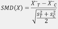
SMD is attractive because it behaves like an effect size: unlike p-values, it does not shrink mechanically with large sample sizes, making it more stable for product-scale datasets. It is also common to look beyond means: variance ratios for continuous covariates, distributional plots, and checks for insufficient overlap (“common support”).

Covariate Balance Table

The table below is illustrative (not a claim about any specific company). It demonstrates a typical reporting pattern: for each covariate, show the treatment/control means (or proportions) and the SMD before and after matching, including the sample sizes. (The true experiment sample size is unspecified per the request.)

Covariate	Stage	n_T	n_C	T mean/prop	C mean/prop	SMD
User tenure (days)	Unmatched	120000	120000	410.00	360.00	0.250
User tenure (days)	Matched	85000	85000	390.00	385.00	0.025
Prior purchase count	Unmatched	120000	120000	9.00	7.00	0.250
Prior purchase count	Matched	85000	85000	8.40	8.20	0.025
Review frequency (reviews/30d)	Unmatched	120000	120000	1.10	0.80	0.300
Review frequency (reviews/30d)	Matched	85000	85000	0.95	0.93	0.020
Electronics category exposure (prop.)	Unmatched	120000	120000	0.42	0.32	0.208
Electronics category exposure (prop.)	Matched	85000	85000	0.38	0.37	0.021
Mobile device (prop.)	Unmatched	120000	120000	0.72	0.62	0.214
Mobile device (prop.)	Matched	85000	85000	0.70	0.69	0.022
US geography (prop.)	Unmatched	120000	120000	0.58	0.50	0.161
US geography (prop.)	Matched	85000	85000	0.55	0.54	0.020

These are the patterns you want to see: substantial reductions in SMD across the board, with the cost that some units (here, illustratively) fall outside overlap and are dropped by matching and/or calipers. That “cost” is not a bug, but it is the dataset telling you where the counterfactual comparison is weak.

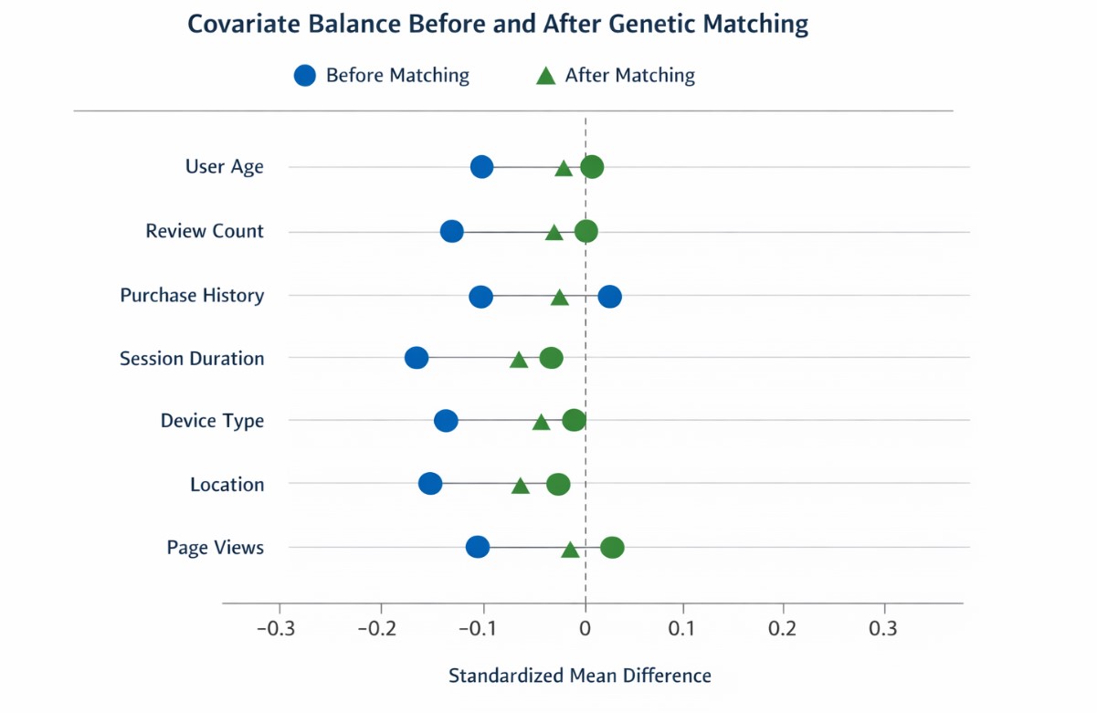
Balance Improvement Chart

A visual “Love plot” style chart is often the fastest way to communicate balance improvement to stakeholders. The figure below plots the absolute SMD before and after matching (the dashed reference line is a commonly used heuristic for detecting meaningful imbalance in applied matching diagnostics). Before/after covariate balance improvement (absolute SMD)

Overlap and Cariance Diagnostics

Even strong SMDs cannot rescue a design with poor overlap. In the propensity score literature, the comparability requirement holds that, within covariate strata, units must have a nontrivial chance of appearing in either group; when this fails, your estimand effectively shifts to the region of overlap.

Use variance ratios as a complementary check because balanced means can still mask meaningful distributional differences. Researchers commonly recommend ratios close to 1 in balance assessments, along with distributional plots. Finally, do not restrict diagnostics to only the covariates you matched on in their raw form: matching guidance recommends checking interactions and nonlinear terms as well, because balance on main-effect means does not guarantee balance on other distributional features.

Estimating Effects after Matching

Once you have a matched dataset, the outcome analysis must align with the matched design and chosen estimand. A straightforward estimator is the difference in mean outcomes across matched treated and matched controls (or weighted analogs if matching weights or replacement are used). If you are using matching as preprocessing, it is common to apply regression adjustment on the matched sample to reduce residual variance and model dependence, consistent with the “preprocess, then analyze” framework. Inference requires care. Matching induces dependence especially with replacement and introduces additional variability from the matching process itself. Established variance estimators in the matching literature, including approaches associated with Abadie and Imbens, account for this structure and should be used.

For product experiments, you also need to account for clustering and repeated-measures realities (e.g., multiple sessions per user): the safest operational move is often to define the unit at the user level for matching and effect estimation, or to use cluster-robust approaches when appropriate. Finally, if primary decisions rely on intent-to-treat A/B results, clearly label matched or exposure-based estimates as secondary estimands. Blurring these distinctions can lead to confusion and unintended “metric shopping.”

Limitations of Genetic Matching for Causal Inference

Genetic matching is powerful, but it is not a magic wand. Principled use requires being direct about limitations:

1. It Only Balances Observed Covariates

Like propensity score methods broadly, matching depends on the assumption that conditioning on the selected pre-treatment covariates is sufficient for comparability. If there are strong unobserved drivers of both exposure to the new review experience and the outcome, matching cannot remove that bias.

2. It can Reveal (and Enforce) Limited Overlap

When overlap is poor, matching will drop units or reuse controls. This is appropriate, but it means the estimand is no longer “all users” unless you design it that way; you are learning about the overlap region.

3. High-Cardinality Categorical Covariates are an Engineering Challenge

Product category and geography can explode dimensionality. You often need pragmatic grouping (category families, country groups) or a hybrid design (exact-match on a few key partitions, then genetic match within partitions).

4. Computation can be Material

The genetic search is iterative, and careful tuning requires you to set population size and generation limits and to monitor convergence. Parallelism is supported and often essential.

5. Reproducibility is Not Optional

Genetic matching contains randomness. MatchIt’s documentation explicitly notes that you must set a seed for reproducibility and that parallel execution requires a parallel-safe seed strategy. At a minimum, reproducibility in a product experimentation context should include: frozen covariate definitions, versioned code, logged matching configuration (calipers, replacement choice, loss function), stored learned weights, and an archived balance report (table + plot) saved as durable artifacts (PNG/SVG).

6. Software and Workflow Tips

In R, the most direct path is Matching::GenMatch() + Matching::Match() (and Matching::MatchBalance()), or MatchIt with method = “genetic” as a higher-level interface. For balance reporting, cobalt provides standardized balance tables and Love plots designed for publication and stakeholder review. If your experimentation stack is Python-first, many teams run matching in R as a reproducible step (e.g., in a containerized job) and pass the matched IDs back to the warehouse for outcome computation. The key is to log everything needed to recreate the match exactly.

Final Thoughts

In complex experimentation environments, exposure-based comparisons can quickly drift from randomized intent into observational territory. Genetic matching for causal inference provides a structured, design-stage solution by optimizing covariate balance before outcomes are analyzed. By clearly defining the estimand, enforcing pre-treatment covariate discipline, and validating balance with diagnostics, teams can strengthen the credibility of their findings. While not a substitute for randomized A/B testing, genetic matching is a powerful complementary tool for improving causal validity in real-world product experiments.

References

Alexis Diamond; Jasjeet S. Sekhon. “Genetic Matching for Estimating Causal Effects: A General Multivariate Matching Method for Achieving Balance in Observational Studies.” Review of Economics and Statistics (2013).
Donald B. Rubin. “For Objective Causal Inference, Design Trumps Analysis.” Annals of Applied Statistics (2008).
Daniel E. Ho; Kosuke Imai; Gary King; Elizabeth A. Stuart. “Matching as Nonparametric Preprocessing for Reducing Model Dependence in Parametric Causal Inference.” Political Analysis (2007).
Stuart, Elizabeth A. “Matching Methods for Causal Inference: A Review and a Look Forward.” Statistical Science (2010).
Austin, Peter C. “Balance Diagnostics for Comparing the Distribution of Baseline Covariates Between Treatment Groups in Propensity-Score Matched Samples.” Statistics in Medicine (2009).

Author Bio: Dharmateja Priyadarshi Uddandarao

Dharmateja Priyadarshi Uddandarao is an accomplished data scientist and statistician, recognized for integrating advanced statistical methods with practical economic applications. He has led projects at leading technology companies, including Capital One and Amazon, applying complex analytical techniques to address real-world challenges. He currently serves as a Senior Data Scientist–Statistician at Amazon.

Quiz Result
Total Questions	Correct Answers	Wrong Answers	Percentage

Executive Summary

The Pre-Balancing Problem in Product Experiments